Bilaterial filter for Photon noise suppression

For the controller in adaptive optics system, the photon shot noise can be a serious issue. But there is a promising results\cite{bilaterialshotnoise} in shot noise filtering using Bilaterial filter. Bilateral filtering was proposed in\cite{tomasibilateral} as a non-iterative method for edge-preserving smoothing.

The MATLAB implementation of bilateral filter can be found here or here.

The bilateral filter is a local filter\cite{aurich1995non,smith1997susan,tomasibilateral} that reduces noise in images while preserving edges by means of non-linear combination of local pixel values. However the problem is to find optimal parameter for the bilateral filter in each case of the signal level.

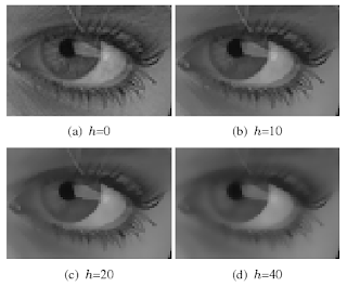
Bilateral filtering using a $5\times5$ square window as $\beta$ and a variable $h$


The bilateral filter replaces a pixel value in an image by a weighted mean of its neighbours considering both their geometric closeness and photometric similarities\cite{bilaterialshotnoise}.

The Gaussian bilateral filter version has a set of parameters that have an important impact on filtering behaviour and performance. The Gaussian bilateral filter is the most used on practice\cite{paris2009fast}:

$v(x) = \frac{1}{C(x)} \sum_{\beta} exp(-\frac{|x-y|^2}{\rho^2}) exp(-\frac{|u(y) - u(x)|^2}{h^2})$

where $\beta$ represents the sliding window, y is a set of 2-D pixel
positions in the sliding window, and x is the 2-D position of
the centred pixel in the sliding window. The u(x) is the intensity
of the pixel at the x position in the original image, v(x) is
the estimated pixel at the x position, $\rho$ and $h$ are the standard deviation of the Gaussian distribution of the geometrical and the intensity weight respectively.

Parameter $\rho$ can be chosen considering the size of the convolution kernel.

Parameter h has to be chosen considering the level of filtering needed for the application.

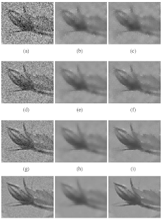
The paper\cite{bilaterialshotnoise} presents the approach of adaptive parameters choice. But it is more interesting to see the actual noise suppression capabilities of the bilateral filter.




From left to right, the first column shows the noisy images, the second column shows the bilateral filtered images with a h parameter fixed to 100, the third column shows the results obtained with our proposed method.


As stated earlier, the bilateral filter smoothing properties
vary with h. Intuitively we can assume that a low h should be preferable in low noise level, whereas a high h may be necessary in high-noise conditions.

REFERENCES:

\bibitem{bilaterialshotnoise}
H.~Phelippeau, H.~Talbot, M.~Akil, and S.~Bara.
\newblock {Shot noise adaptive bilateral filter}.
\newblock pages 864--867, 2008.

\bibitem{tomasibilateral}
C.~Tomasi and R.~Manduchi.
\newblock {Bilateral filtering for gray and color images}.
\newblock pages 839--846, 1998.

\bibitem{aurich1995non}
V.~Aurich and J.~Weule.
\newblock {Non-linear gaussian filters performing edge preserving diffusion}.
\newblock pages 538--545, 1995.

\bibitem{smith1997susan}
S.M. Smith and J.M. Brady.
\newblock {SUSAN - A new approach to low level image processing}.
\newblock {\em International journal of computer vision}, 23(1):45--78, 1997.

\bibitem{paris2009fast}
S.~Paris and F.~Durand.
\newblock {A fast approximation of the bilateral filter using a signal
processing approach}.
\newblock {\em International journal of computer vision}, 81(1):24--52, 2009.

A little note on Shack-Hartmann wavefront sensor

A well-known Hartmann test\cite{hartmann1900} devised initially for telescope optics control was adapted for adaptive optics. The design of this sensor was based on an aperture array that had been developed by Johannes Franz Hartmann\cite{platt2001history} as a means to trace individual rays of light through the optical system of a large telescope, thereby testing the quality of the image\cite{hartmann1900}. In the late 1960s Shack and Platt\cite{shackhartmproduction} modified a Hartmann screen by replacing the apertures in an opaque screen with an array of lenslets.


It is interesting that the construction of SH WFS is simple yet effective; in fact, first lenslet arrays were kithcen-made\cite{platt2001history}:

Platt made a mount for compression, moulding a 1-mm-thick square plate of optical grade thermal plastic (Plexiglass) between the two Cervet squares. [...] Each heating and cooling cycle in the moulding process took several hours. So, Platt decided to work all day and most of the night in his wife's kitchen. His wife's electric knife sharpener was used to trim the Plexiglass plates. Her apron and oven mittens were also used to remove the moulds from the oven. After a few weeks, the process was perfected and good quality lens arrays were being produced. For at least the next 5 years, all lens arrays used in Shack-Hartmann wavefront sensors were made by Platt in his wife's kitchen.

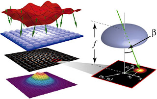
The principle of the Shack-Hartmann (SH) wavefront sensor (WFS) is the following. An image of the exit pupil is projected onto a lenslet array. Each lens takes a small part of the aperture (sub-aperture), and forms an image of the source. When an incoming wavefront is planar, all images are located in a regular grid defined by the lenslet array geometry. As soon as the wavefront is distorted, images become displaced from their nominal positions. Displacements of image centroids in two orthogonal directions $x,y$ are proportional to the average wavefront slopes in $x,y$ over the sub-apertures.


Centroiding
For a sampled light intensity $I_{i,j}$, positions of spots $x_{c_k}$ and $y_{c_k}$ are:

$$ x_{c_k} = \frac{\sum_{i,j} x_{i,j}I_{i,j}}{\sum_{i,j} I_{i,j}},\,\,\,\,
y_{c_k} = \frac{\sum_{i,j} y_{i,j}I_{i,j}}{\sum_{i,j} I_{i,j}},
$$

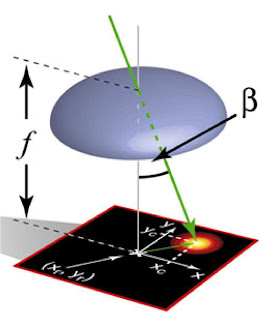
Resulting local direction angle $\beta$:
$$
\beta_x \approx (x_{c_k} - x_{r_k})\frac{L_x}{f},\,\,\,\,
\beta_y \approx (y_{c_k} - y_{r_k})\frac{L_y}{f},
$$

where $L_x$ is a size of the photosensor's pixel and $f$ is the focus length of the lenslet.


\vspace{3ex}\textit{Advantages}: predictable results, simple and effective construction, ability to simultaneously determine $x$ and $y$ slopes.

\vspace{3ex}\textit{Disadvantages}: centroiding algorithm is computationally-intensive.

\vspace{3ex}Shack-Hartmann wavefront sensor is the most popular: its precision and accuracy can be scaled over a huge range through the choice of lenslet array and detector.



Typical WFS SH characteristics
Typical parameters for the Shack-Hartmann sensor in the year 2010 are:

• Aperture Size 5.95 mm x 4.76 mm. Max.
• Camera Resolution 1280 x 1024 Pixels Max.
• Pixel Size $4\dots5.5 \mu$m
• lenslet size 300$\mu m$
• lenslet focus distance 7 mm
• Number of Subapertures $\leq 150$

References \begin{thebibliography}{1}

\bibitem{hartmann1900}
J.~Hartmann.
\newblock {Bemerkungen {\"u}ber den Bau und die Justirung von Spektrographen}.
\newblock {\em Z. Instrumentenkd}, 20:47, 1900.

\bibitem{platt2001history}
B.C. Platt.
\newblock {History and principles of Shack-Hartmann wavefront sensing}.
\newblock {\em Journal of Refractive Surgery}, 17(5):573--577, 2001.

\bibitem{shackhartmproduction}
R.V. Shack and B.C. Platt.
\newblock {Production and use of a lenticular Hartmann screen}.
\newblock {\em J. Opt. Soc. Am}, 61(5):656, 1971.

\end{thebibliography}

When the Poisson distribution can be approximated as Gaussian?

In many articles that deal with noise, and especially in photosensors, there is a usual mantra assume the noise as a Gaussian distributed. Such mantra is said even to processes that are Poissonian by the very nature (photon shot noise). The question: ``how many arrivals can justify the Gaussian approximation?'' is usually answered in vague term ``many''. Well, how many!?

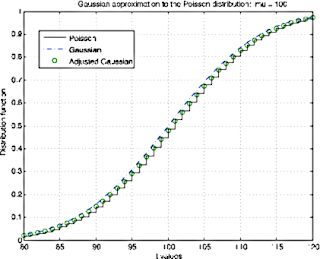
Good question. Some authors say\cite{mendenhallstatistics} that more then 1000 arrival events can be considered as Gaussian. And it seems to be reasonable, as shown [the picture from here]:

The approximation of Poisson distribution by Gaussian is performed usually to simplify the calculations. However, the approximation is not simple. In\cite{poisson2gaussapprox} was shown that the usual approximation of a Poisson density function with mean $m$ by a Gaussian density function with mean $\mu$ and variance $\sigma$ both equal to $m$ is in general not satisfactory for error-rate calculations. A short letter to IEEE Transactions describes a modified Gaussian approximation to a Poisson distribution which, unlike the usual Gaussian approximation, gives good agreement on the tails of the distribution.

We can express Poisson distribution $p(n, m)$ in terms of Gaussian $g(n,m)$ as follows\cite{poisson2gaussapprox}:

$$p(n,m) = \left(\frac{1}{\sqrt{2\pi m}}\right)^{\frac{1}{1+\alpha}} \exp\left[ -\frac{\beta}{1+\alpha} - \frac{(n-m)^2}{2m(1+\alpha)} \right] $$

Thus a Gaussian that better approximates Poisson $p(n, m)$ on the tails has the same mean as $p(n, m)$ but has variance $m(1 + \alpha)$.

The parameters $\alpha$ and $\beta$ can be expressed via $\mu$ as:

$\alpha = (0.080\mu^2 - 0.230\mu + 1.260)^{-2}$

and

$\beta = (0.0667\mu^2 -0.3933\mu + 0.810)^{-1}$

References:

\begin{thebibliography}{1}

\bibitem{mendenhallstatistics}
W.~Mendenhall and T.~Sincich.
\newblock {Statistics for Engineering and the Sciences}.
\newblock 2006.

\bibitem{poisson2gaussapprox}
W.M. Hubbard.
\newblock The approximation of a poisson distribution by a gaussian
distribution.
\newblock {\em Proceedings of the IEEE}, 58(9):1374 -- 1375, 1970.

\end{thebibliography}

Small Radiometry FAQ

Let's define the radiometry and photometry units for the light source. Radiometry is the measurement of optical radiation, which is electromagnetic radiation within the frequency range between $3\times10^{11}$ and $3\times10^{16}$ Hz ($\lambda \in 0.01 .. 1000 \mu m$). Typical units encountered are Watt/$m^2$ and photons/s-steradian[1].

Photometry is the measurement of light, which is defined as electromagnetic radiation that is detectable by the human eye. It is restricted to the wavelength range from $\lambda \in 0.36 .. 0.83 \mu m$ [1]. Photometry is radiometry that is weighted by the spectral response of the eye.


Light sources
The light is generated by the source with known radiance and wavelength $\lambda$. Irradiance is known for the sensor in Watt/$m^2$ [2]. There are two types of light sources: lambertian and isotropic[3]. Both terms mean the same in all directions but they are not interchangeable.

Isotropic implies a spherical source that radiates the same in all directions, i.e., the intensity (W/sr) is the same in all directions. We often encounter the phrase ``isotropic point source'', however there can be no such thing because the energy density
would have to be infinite. But a small, uniform sphere comes very close. The best
example is a globular tungsten lamp with a milky white diffuse envelope. A distant star can be considered an isotropic point source.

Lambertian refers to a flat radiating surface. It can be an active surface or a passive, reflective surface. Here the intensity falls off as the cosine of the
observation angle with respect to the surface normal, that is Lambert's law[4]. The radiance
(W/$m^2$-sr) is independent of direction.



Radiometric units
Radiometric units can be divided into two conceptual areas: those having to do with
power or energy, and those that are geometric in nature. The first two are:

Energy is an SI derived unit, measured in joules (J). The recommended symbol for
energy is $Q$. An acceptable alternate is W[2].

Power (radiant flux) is another SI derived unit. It is the rate of flow
(derivative) of energy with respect to time, $dQ/dt$, and the unit is the watt (W). The
recommended symbol for power is $\Phi$. An acceptable alternate is P.

Now we incorporate power with the geometric quantities area and solid angle.

Irradiance (flux density) is another SI derived unit and is measured in W/$m^2$.
Irradiance is power per unit area incident from all directions in a hemisphere \textit{onto a
surface} that coincides with the base of that hemisphere. The symbol for irradiance is $E$ and the symbol for radiant exitance is $M$. Irradiance is the derivative of power
with respect to area, $d\Phi/dA$. The integral of irradiance or radiant exitance over
area is power.

Radiance is the last SI derived unit we need and is measured in W/$m^2$-sr. Radiance
is power per unit projected area per unit solid angle. The symbol is L. Radiance is
the derivative of power with respect to solid angle and projected area, $d\Phi/d\omega dA
cos(\theta)$, where $\theta$ is the angle between the surface normal and the specified direction. The integral of radiance over area and solid angle is power.

A great deal of confusion concerns the use and misuse of the term intensity. Some
use it for W/sr, some use it for W/$m^2$ and others use it for W/$m^2$-sr. It is quite
clearly defined in the SI system, in the definition of the base unit of luminous
intensity, the candela. For an extended discussion see Ref.[5].


Astronomical Magnitudes
In astronomy, absolute magnitude (also known as absolute visual magnitude when measured in the standard V photometric band) measures a celestial object's intrinsic brightness. To derive absolute magnitude from the observed apparent magnitude of a celestial object its value is corrected from distance to its observer. One can compute the absolute magnitude $M$, of an object given its apparent magnitude $m\,$ and luminosity distance $D_L\,$:

$M = m - 5 ((\log_{10}{D_L}) - 1)\, $

where $D_L\,$ is the star's luminosity distance in parsecs, wherein 1 parsec is approximately 3.2616 light-years. The dimmer an object appears, the higher its apparent magnitude.
The apparent magnitude in the band x can be defined as (noting that $\log_{\sqrt[5]{100}} F = \frac{\log_{10} F }{\log_{10} 100^{1/5}} = 2.5\log_{10} F$)


$m_{x}= -2.5 \log_{10} (F_x/F_x^0)\,$

where $F_x\,$ is the observed flux in the band $x$, and $F_x^0$ is a reference flux in the same band x, such as the Vega star's for example.


Conversion to photons
Photon quantities of light energy are also common. They are related to the radiometric quantities by the relationship $Q_p = hc/\lambda$ where $Q_p$ is the energy of a photon at wavelength $\lambda$, $h$ is Planck's constant and $c$ is the velocity of light. At a wavelength of $1 \mu m$, there are approximately $5\times10^{18}$ photons per second in a watt. Conversely, a single photon has an energy of $2\times10^{-19}$ joules (W s) at $\lambda = 1 \mu m$.

References

1

J.M. Palmer and L. Carroll.
Radiometry and photometry FAQ, 1999.

2

C. DeCusatis.
Handbook of applied photometry.
American Institute of Physics, 1997.

3

The basis of physical photometry.
Technical report, CIE Technical Report 18.2, 1983.

4

J.H. Lambert.
Photometria sive de mensura de gratibus luminis, colorum et umbrae.
Eberhard Klett, 2, 1760.

5

J.M. Palmer.
Getting intense on intensity.
Metrologia, 30:371, 1993.

Autoregressuve (AR) models of random sequences

The ideas behind Autoregressive model are considered in this digest. Examples of describing the autoregressive model are evaluated.

Autoregressive model of a stochastic signal in a nutshell
Assume we have a noise-alike discrete sequence $y[n]$ that we want to study. We can describe the signal in terms of autocorrelation or power spectrum density, but we can also describe it in the other way. We can actually describe the noised signal $y[n]$ as a result of passing a white noise $x[n]$ through a filter $h[n]$. The filter $h[n]$ can be described in Z-domain as following:

$H(z) = \frac{B(z)}{A(z)} = \frac{\sum\limits_{k=0}^{q} b_k z^{-k} }{1+ \sum\limits_{k=0}^{p} a_k z^{-k} }$

that is a stable shift-invariant linear system with $p$ poles and $q$ zeros. The autoregressive (AR) model is a case of the ARMA and is the following:

$H(z) = \frac{b_0}{1+ \sum\limits_{k=0}^{p} a_k z^{-k} }$

where $a_1, \dots, a_p$ are the parameters of the model. We can think\cite{ramadanadaptivefiltering} of the signal $y[n]$ being studied as a result of passing the white noise $x[n]$ with known variance $\sigma_x^2$ through the filter $H[z]$.

The autocorrelation function $y[n]$ and the parameters of the filter $H[z]$ are related via Yule-Walker equation:

$R_{yy}[k] + \sum_{m=1}^p a_m R_{yy}[k-m] = \sigma_x^2 b_0^2 \delta_{m,0},$

where $m = 0, ... , p,$ yielding $p+1$ equations. Those equations are usually written in matrix form:

$\left[ \begin{matrix}
R_{yy}(0) & R_{yy}(-1) & \dots R_{yy}(-p) \\
R_{yy}(1) & R_{yy}(0) & \dots R_{yy}(-p+1) \\
\vdots & \vdots & \vdots \\
R_{yy}(p) & R_{yy}(p-1)& \dots R_{yy}(0) \\
\end{matrix} \right]
\left[ \begin{matrix}
1 \\ a_1 \\ \vdots \\ a_p
\end{matrix}\right]
= \sigma_x^2 b_0^2
\left[ \begin{matrix}
1 \\ 0 \\ \vdots \\ 0
\end{matrix}\right]$

and we need to solve this matrix equation for coefficients $a_1 \dots a_p$. The above equations provide the way for estimation of the parameters of an AR(p) model. In order to solve the matrix equation, we must replace the theoretical covariances with estimated values such as $R_{yy}(0)$.


A note of Toeplitz matrices
When we study a signal and calculate its autocorrelation sequence, we got a vector. In order to use these data in solving the matrix equation, we need to convert the autocorrelation vector into matrix. That can be performed by Toeplitz matrices. A Toeplitz matrix is a matrix in which each descending diagonal from left to right is constant:

$\begin{bmatrix} a & b & c & d & e \\ f & a & b & c & d \\ g & f & a & b & c \\ h & g & f & a & b \\ i & h & g & f & a \end{bmatrix}.$

A Toeplitz matrix is defined by one row and one column. A symmetric Toeplitz matrix is defined by just one row. In order to generate the Toeplitz matrix, one can use \textbf{toeplitz} function in MATLAB that generates Toeplitz matrices given just the row or row and column description.

In the example below we will generate the autocorrelation matrix from the vector using Toeplitz matrices. Consider we have the autocorrelation vector of the observed signal $y[n]$ over the lag range \textit{[-maxlags:maxlags]}. The output vector $r_{yy}$ will have the length \textit{2*maxlags+1}:
\begin{verbatim}
[r_yy, lags] = xcorr(y,y,xcorr_maxlags,'biased');
\end{verbatim}

The output will be autocorrelation vector like this:
$r_{yy} = 0.7066 \,\,\,\, 0.7116 \,\,\,\, 0.7176 \,\,\,\,0.7147 \,\,\,\, 0.7018 \,\,\,\, 0.6954 \,\,\,\, 0.7029 \,\,\,\, 0.7208 \,\,\,\, 0.7323 \,\,\,\, 0.7245$

Then we need to make a autocorrelation matrix - use the Toeplitz matrices:
\begin{verbatim}
R = toeplitz(r_yy(1,1:acorr_matrix_size)); %% create the autocorr. matrix
\end{verbatim}
The result will be like:

$R =
\left[ \begin{matrix}
0.7066& 0.7116& 0.7176& 0.7147& 0.7018& 0.6954 \\
0.7116& 0.7066& 0.7116& 0.7176& 0.7147& 0.7018 \\
0.7176& 0.7116& 0.7066& 0.7116& 0.7176& 0.7147 \\
0.7147& 0.7176& 0.7116& 0.7066& 0.7116& 0.7176 \\
0.7018& 0.7147& 0.7176& 0.7116& 0.7066& 0.7116 \\
0.6954& 0.7018& 0.7147& 0.7176& 0.7116& 0.7066 \\
\end{matrix} \right]$

That is how we can make the autocorrelation matrix from the autocorrelation vector.


Example of the Autoregressive model
Consider the example in MATLAB from the book \cite{ramadanadaptivefiltering}. First of all, let's generate the signal $y[n]$ from the white noise (it is a simulation of the real signal).
\begin{verbatim}
x = 1.0*(rand(1,signal_length) - 0); % x is a White Gaussian Noise.
y = filter(1, [1 -0.9 0.5], x); % here y is observed (filtered) signal.
\end{verbatim}
The \textbf{filter} function filters \textbf{y = filter(b,a,X)} the data in vector \textbf{X} with the filter described by numerator coefficient vector \textbf{b} and denominator coefficient vector \textbf{a} that is:

$y(n) = b(1)*x(n) + b(2)*x(n-1) + ... + b(nb+1)*x(n-nb) - a(2)*y(n-1) - ... - a(na+1)*y(n-na)$


Any WSS process $y[n]$ can be represented as the output of filter $h[n]$ that is driven by noise x[n]. Using that filter coefficients (arbitrary chosen - we just need to generate the signal), we design the signal which we are going to study. Then we describe the signal $y[n]$ in terms of filter function defined by AR coefficients.

In order to solve Yule-Walker equations, we need to find the autocorrelation function of the signal $y[n]$:

\begin{verbatim}
[r_yy, lags] = xcorr(y,y,xcorr_maxlags,'biased'); %% autocorrelation vector of the observed signal y[n]
R = toeplitz(r_yy(1,1:acorr_matrix_size)); %% create the smaller autocorrelation matrix
\end{verbatim}

We used the Toeplitz matrix, as described above, to obtain the autocorrelation matrix. The variable \verb|acorr_matrix_size| is for setting the size of the autocorrelation matrix, which is also setting the order of the filter H(z):

$H(z) = \frac{b_0}{1+ \sum\limits_{k=0}^{p} a_k z^{-k} }$

OK, now we need to find the coefficients $a_1 \dots a_p$ so we need to find the inverse autocorrelation matrix:

\begin{verbatim}
R_inv = pinv(R); %% R_inv is the inverse of R
\end{verbatim}

First element of the $R_{yy}$ is the $b_0^2$ coefficient that is needed for the filter $H(z)$:
\begin{verbatim}
b0_squared = 1/R_inv(1,1); %% this is a variance of the process R_yy(0)
b0 = sqrt(b0_squared); %% find b0 that is \sqrt{R_yy(0)}.
\end{verbatim}
Using these data, we can find the AR coefficients $a_1 \dots a_p$:
\begin{verbatim}
a = b0_squared*R_inv(2:acorr_matrix_size,1); %%% find the AR coefficients
\end{verbatim}

Then we should denote the order of the filter that is $H(z) = \frac{b_0}{1+a_1z_{-1}+...+a_kz^{-k}}$ by denoting the number of autocorrelation coefficients used. Finally, we can calculate the filter:
\begin{verbatim}
H = b0./(fft([1 a'],filter_fft_length)); %% H is the frequency response of the filter
\end{verbatim}
Now we can describe the process y[n] in terms of the autoregressive model coefficients $a_1 \dots a_p$.

Voice-coil actuators in adaptive optics

Voice-coil actuators are a special form of electric motor, capable of moving an inertial load at extremely high accelerations and relocating it to an accuracy of millionths of an inch over a limited range of travel. Motion may be in a straight line (linear actuators) or in an arc (rotary, or swing-arm actuators)\cite{emdesignandactuators}. They are called "voice coil actuators" because of their common use in loudspeakers.


When electric current flows in a conducting, wire which is in a magnetic field, a Lorentz force is produced on the conductor which is at right angles to both the direction of current and magnetic field. The voice coil actuators are nothing but the technical manifestation of the Lorentz force principle, according to which "power current carrying windings of electrical conductivity is directly proportional to the strength of the magnetic field and current."


The electromechanical conversion mechanism of a voice coil actuator is governed by the Lorentz Force: if a current-carrying conductor is placed in a magnetic field, a force of magnitude
$F = kBLIN$
will act upon it, where:

• k - Constant
• F - Force
• B - Magnetic flux density
• I - Current
• L - Length of a conductor
• N - Number of conductors

In its simplest form, a linear voice coil actuator is a tubular coil of wire situated within a radially oriented magnetic field. The field is produced by permanent magnets embedded on the inside diameter of a ferromagnetic cylinder, arranged so that the magnets ``facing'' the coil are all of the same polarity.



Note that when the current direction is reversed, then (assuming that the direction of B is unchanged), the direction of the force is reversed. The reversible force of a voice coil actuator is an advantage over the force of moving iron actuators of the preceding sections, which is directed to attract the iron armature toward the iron stator regardless of the direction of the current. Another advantage over solenoid actuators is that voice coil force is much more independent of armature position and is proportional to current. A minor disadvantage is that the voice coil current must be supplied via a flexible lead, and thus the proper stranded wire must be selected for reliable long-term operation\cite{brauer2006magnetic}.

The electromagnetic (EM) driver consists of a coil moving in a magnetic field and driving a piston against a cylindrical spring. A permanent magnet with pole pieces is used to transmit the force to the backplate\cite{dmforallseasons}. Voice-coil actuators are electromagnetic devices which produce accurately controllable forces over a limited stroke with a single coil or phase. They are also often called linear actuators, a name also used for other types of motors\cite{voicecoilsbasics}. Because the moving parts of the speaker must be of low mass (to accurately reproduce high-frequency sounds), voice coils are usually made as light weight as possible, making them delicate. Passing too much power through the coil can cause it to overheat (caused by ohmic heating).

The single phase linear voice coil actuator allows direct, cog-free linear motion that is free from the backlash, irregularity, and energy loss that results from converting rotary to linear motion\cite{voicecoilsactbasics}.


References:

\begin{thebibliography}{1}

\bibitem{emdesignandactuators}
Jr. George P.~Gogue, Joseph J.~Stupak.
\newblock {\em Theory \& Practice of Electromagnetic Design of DC Motors \&
Actuators (CHAPTER 11, ACTUATORS)}.
\newblock G2 Consulting, Beaverton, OR 97007.

\bibitem{brauer2006magnetic}
J.R. Brauer.
\newblock {Magnetic actuators and sensors}.
\newblock 2006.

\bibitem{dmforallseasons}
R.~H. Freeman and J.~E. Pearson.
\newblock Deformable mirrors for all seasons and reasons.
\newblock {\em Applied Optics}, 21(4):580--588, 1982.

\bibitem{voicecoilsbasics}
George~P. Gogue and Jr. Joseph J.~Stupak.
\newblock Voice-coil actuators.
\newblock Technical report, G2 Consulting, Beaverton, OR 97005, 2007.

\bibitem{voicecoilsactbasics}
B.~Black, M.~Lopez, and A.~Morcos.
\newblock {Basics of Voice Coil Actuators}.
\newblock {\em PCIM-VENTURA CA-}, 19:44--44, 1993.

\end{thebibliography}

DNA as a programming code

Just a short note not to forget: for quite a long time, one idea is wandering in my head. I can probably entitle it something like DNA as a compiled code: An engineering look on the biological problem.

In essence, the idea is the following. We used to make the devices that are either monolythic or disassembleable. That's fine, but such devices must be made at once and they are not capable of self-maintanece or self-development. What if we can write a computer-alike code that can be compilled to DNA? DNA can be a kind of compiled code, but it is possible to develop a programming language that allows to describe the properties of living organisms and compile it into DNA. It is possible to go from blindly copying and editing of DNA to a meaningful design of biological devices.

Some of ideas like that are being explored. Recently there were an article ''Programmable Bacteria''.

In research that further bridges the biological and digital world, scientists at the University of California, San Francisco have created bacteria that can be programmed like a computer. Researchers built 'logic gates' ? the building blocks of a circuit ? out of genes and put them into E. coli bacteria strains. The logic gates mimic digital processing and form the basis of computational communication between cells, according to synthetic biologist Christopher A. Voigt.