Monday, March 14, 2011

Adding a probability distribution to another: superimpose the probability distribution

We all learned some probability theory at Uni, but the learning pure theory is one thing, and application of it is slightly different. There is learning, understanding and there is an acceptance, as O'Brien from 1984 has told. The topic of this post is how to superimpose two (or more) distributions.

Introduction
For instance, we have a skewed probability density function and the data generated according to it. Let it be Log-Normal distribution:

$p_{LogNorm}(x;\mu, \sigma) = \frac{1}{x\sqrt{2\pi\sigma^2}}\, e^{-\frac{\left(\ln x-\mu\right)^2}{2\sigma^2}}$

with parameters $\mu = 4.0246$ and $\sigma = 0.0350$ respectively. The data looks like:
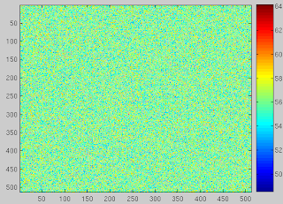
OK, so far so good: the data is noisy and have values from about 50 to about 64, that is in consistency with the probability probability density function:
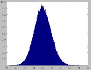
The pdf was numerically estimated using hist function in MATLAB.

The Problem:
I need to make a new pdf that is superimposed by the uniform distribution. The idea is to make a distribution with very long "tail". Well, we can do it accurately, using theoretical expressions of sum of random variables (see, for instance, Probability and random processes by Stark and Woods, Chapter 3). But after all, we need to generate the data using it and not just tinker with it.


The solution
Let's say, we need to add some uniform distribution in order to make the "tail" of summary distribution longer. OK, we can easily generate uniform distribution using rand function in MATLAB or Octave. Generate a uniform distribution of random numbers on a specified interval [a,b]. To do this, multiply the output of rand by (b-a) then add a. Here is MATLAB code:
Isize = 256;
a=5;
b=50;
I = a + (b-a)*rand(Isize);
Now it is not obvious: if we just add two distributions (either in spatial domain or in Fourier domain using point-wise addition), we will get wrong result:

What has happenned? Well, because this is uniform distribution, it just wiped out our gentle Log-Normal data. Hence we need to attenuate the amount of the uniform distribution that we add.

One solution is to add, say, every second data point. Nice idea, but not clever: our data will be periodic that is not desirable. The better solution is to generate another uniform distribuiton [0,1] and make it like a mask for addition of desired data points.

In order to attenuate the influence of the other distribution, we need to add only a few point from the other distribution. Here is the example:

z = ones(Isize); %% creating a mask of the adding new pdf.
addition_percentage = 0.6;
z = rand(Isize,Isize);
z(z>addition_percentage) = 0;

%%% Erasing the unnecessary points from the other distribution
I = I.*z;
Here our mask will be like:

0 0 0.1157 0.2088 0.5074

0.3981 0 0.3826 0.3936 0.1435

0 0.0476 0.5989 0.5155 0.5239

0 0 0 0.4117 0

0 0 0.0858 0 0

0 0.4345 0.4846 0.4592 0

0 0.4591 0.3690 0.1043 0

We can use ceil(z) to make it just 0 or 1, but in our case we want the "tail" to decay. Multiplication of two uniform distribution is not a longer uniform distribution, as one might think :-) It will be triangular-shaped and, if we continue to multiply it more, will tend to be Gaussian, as followed by CLT:
The Central Limit Theorem (CLT) states conditions under which the mean of a sufficiently large number of independent and identically distributed random variables, each with finite mean and variance, will be approximately normally distributed.
So then we just add:
I2 = I+Ilong;
where I is uniform distribution multiplied by uniform mask (now will be triangular-like), and Ilong is long-tailed distribution. The result pleases the eye, the mind and the soul:
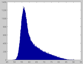
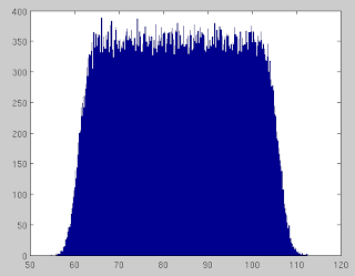
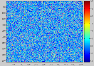
That's exactly what we desired, and the data is appropriate:
Now it's a good time to write a huge article to SIAM Journal entitled "Recent ground-breaking advances in Advanced Probability Theory" :-)


Various thoughts and jots

The sum of two normal distributions is itself a normal distribution:

N(mean1, variance1) + N(mean2, variance2) ~ N(mean1 + mean2, variance1 + variance2)

This is all on wikipedia page.

Be careful that these really are variances and not standard deviations.
Monday, March 7, 2011

Bilaterial filter for Photon noise suppression

For the controller in adaptive optics system, the photon shot noise can be a serious issue. But there is a promising results\cite{bilaterialshotnoise} in shot noise filtering using Bilaterial filter. Bilateral filtering was proposed in\cite{tomasibilateral} as a non-iterative method for edge-preserving smoothing.

The MATLAB implementation of bilateral filter can be found here or here.

The bilateral filter is a local filter\cite{aurich1995non,smith1997susan,tomasibilateral} that reduces noise in images while preserving edges by means of non-linear combination of local pixel values. However the problem is to find optimal parameter for the bilateral filter in each case of the signal level.

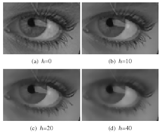
Bilateral filtering using a $5\times5$ square window as $\beta$ and a variable $h$


The bilateral filter replaces a pixel value in an image by a weighted mean of its neighbours considering both their geometric closeness and photometric similarities\cite{bilaterialshotnoise}.

The Gaussian bilateral filter version has a set of parameters that have an important impact on filtering behaviour and performance. The Gaussian bilateral filter is the most used on practice\cite{paris2009fast}:

$v(x) = \frac{1}{C(x)} \sum_{\beta} exp(-\frac{|x-y|^2}{\rho^2}) exp(-\frac{|u(y) - u(x)|^2}{h^2})$

where $\beta$ represents the sliding window, y is a set of 2-D pixel
positions in the sliding window, and x is the 2-D position of
the centred pixel in the sliding window. The u(x) is the intensity
of the pixel at the x position in the original image, v(x) is
the estimated pixel at the x position, $\rho$ and $h$ are the standard deviation of the Gaussian distribution of the geometrical and the intensity weight respectively.

Parameter $\rho$ can be chosen considering the size of the convolution kernel.

Parameter h has to be chosen considering the level of filtering needed for the application.

The paper\cite{bilaterialshotnoise} presents the approach of adaptive parameters choice. But it is more interesting to see the actual noise suppression capabilities of the bilateral filter.


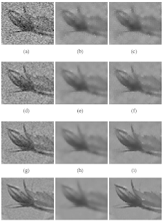
From left to right, the first column shows the noisy images, the second column shows the bilateral filtered images with a h parameter fixed to 100, the third column shows the results obtained with our proposed method.


As stated earlier, the bilateral filter smoothing properties
vary with h. Intuitively we can assume that a low h should be preferable in low noise level, whereas a high h may be necessary in high-noise conditions.


REFERENCES:

\bibitem{bilaterialshotnoise}
H.~Phelippeau, H.~Talbot, M.~Akil, and S.~Bara.
\newblock {Shot noise adaptive bilateral filter}.
\newblock pages 864--867, 2008.

\bibitem{tomasibilateral}
C.~Tomasi and R.~Manduchi.
\newblock {Bilateral filtering for gray and color images}.
\newblock pages 839--846, 1998.

\bibitem{aurich1995non}
V.~Aurich and J.~Weule.
\newblock {Non-linear gaussian filters performing edge preserving diffusion}.
\newblock pages 538--545, 1995.

\bibitem{smith1997susan}
S.M. Smith and J.M. Brady.
\newblock {SUSAN - A new approach to low level image processing}.
\newblock {\em International journal of computer vision}, 23(1):45--78, 1997.

\bibitem{paris2009fast}
S.~Paris and F.~Durand.
\newblock {A fast approximation of the bilateral filter using a signal
processing approach}.
\newblock {\em International journal of computer vision}, 81(1):24--52, 2009.

Wednesday, March 2, 2011

A little note on Shack-Hartmann wavefront sensor

A well-known Hartmann test\cite{hartmann1900} devised initially for telescope optics control was adapted for adaptive optics. The design of this sensor was based on an aperture array that had been developed by Johannes Franz Hartmann\cite{platt2001history} as a means to trace individual rays of light through the optical system of a large telescope, thereby testing the quality of the image\cite{hartmann1900}. In the late 1960s Shack and Platt\cite{shackhartmproduction} modified a Hartmann screen by replacing the apertures in an opaque screen with an array of lenslets.


It is interesting that the construction of SH WFS is simple yet effective; in fact, first lenslet arrays were kithcen-made\cite{platt2001history}:
Platt made a mount for compression, moulding a 1-mm-thick square plate of optical grade thermal plastic (Plexiglass) between the two Cervet squares. [...] Each heating and cooling cycle in the moulding process took several hours. So, Platt decided to work all day and most of the night in his wife's kitchen. His wife's electric knife sharpener was used to trim the Plexiglass plates. Her apron and oven mittens were also used to remove the moulds from the oven. After a few weeks, the process was perfected and good quality lens arrays were being produced. For at least the next 5 years, all lens arrays used in Shack-Hartmann wavefront sensors were made by Platt in his wife's kitchen.
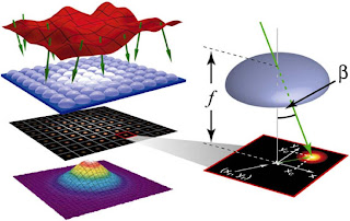
The principle of the Shack-Hartmann (SH) wavefront sensor (WFS) is the following. An image of the exit pupil is projected onto a lenslet array. Each lens takes a small part of the aperture (sub-aperture), and forms an image of the source. When an incoming wavefront is planar, all images are located in a regular grid defined by the lenslet array geometry. As soon as the wavefront is distorted, images become displaced from their nominal positions. Displacements of image centroids in two orthogonal directions $x,y$ are proportional to the average wavefront slopes in $x,y$ over the sub-apertures.


Centroiding
For a sampled light intensity $I_{i,j}$, positions of spots $x_{c_k}$ and $y_{c_k}$ are:

$$ x_{c_k} = \frac{\sum_{i,j} x_{i,j}I_{i,j}}{\sum_{i,j} I_{i,j}},\,\,\,\,
y_{c_k} = \frac{\sum_{i,j} y_{i,j}I_{i,j}}{\sum_{i,j} I_{i,j}},
$$

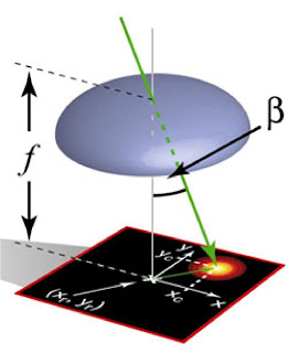
Resulting local direction angle $\beta$:
$$
\beta_x \approx (x_{c_k} - x_{r_k})\frac{L_x}{f},\,\,\,\,
\beta_y \approx (y_{c_k} - y_{r_k})\frac{L_y}{f},
$$

where $L_x$ is a size of the photosensor's pixel and $f$ is the focus length of the lenslet.


\vspace{3ex}\textit{Advantages}: predictable results, simple and effective construction, ability to simultaneously determine $x$ and $y$ slopes.

\vspace{3ex}\textit{Disadvantages}: centroiding algorithm is computationally-intensive.

\vspace{3ex}Shack-Hartmann wavefront sensor is the most popular: its precision and accuracy can be scaled over a huge range through the choice of lenslet array and detector.


Typical WFS SH characteristics

Typical parameters for the Shack-Hartmann sensor in the year 2010 are:
  • Aperture Size 5.95 mm x 4.76 mm. Max.
  • Camera Resolution 1280 x 1024 Pixels Max.
  • Pixel Size $4\dots5.5 \mu$m
  • lenslet size 300$\mu m$
  • lenslet focus distance 7 mm
  • Number of Subapertures $\leq 150$


References \begin{thebibliography}{1}

\bibitem{hartmann1900}
J.~Hartmann.
\newblock {Bemerkungen {\"u}ber den Bau und die Justirung von Spektrographen}.
\newblock {\em Z. Instrumentenkd}, 20:47, 1900.

\bibitem{platt2001history}
B.C. Platt.
\newblock {History and principles of Shack-Hartmann wavefront sensing}.
\newblock {\em Journal of Refractive Surgery}, 17(5):573--577, 2001.

\bibitem{shackhartmproduction}
R.V. Shack and B.C. Platt.
\newblock {Production and use of a lenticular Hartmann screen}.
\newblock {\em J. Opt. Soc. Am}, 61(5):656, 1971.

\end{thebibliography}
Related Posts Plugin for WordPress, Blogger...