Wednesday, October 12, 2011
Compressed sensing: notes and remarks
The idea of Compressed Sensing
The basic idea of CS [1] is that when the image of interest is very sparse or highly compressible in some basis, relatively few well-chosen observations suffice to reconstruct the most significant nonzero components. It can be also considered as projecting onto incoherent measurement ensembles [2]. Such an approach should be directly applied in the design of the detector. Devising an optical system that directly “measures” incoherent projections of the input image would provide a compression system that encodes in the analog domain.
Rather than measuring each pixel and then computing a compressed representation, CS suggests that we can measure a “compressed” representation directly.
The paper [1] provides a very illustrative example of searching the bright dot on a black background: instead of full comparison (N possible locations), the CS allows to do it in M=log2(N) binary measurements using binary masks.
The key insight of CS is that, with slightly more than K well-chosen measurements, we can determine which coefficients of some basis are significant and accurately estimate their values.
A hardware example of Compressed sensing
An example of a CS imager is the rice single-pixel camera developed by Duarte et al [3,4]. This architecture uses only a single detector element to image a scene. A digital micromirror array is used to represent a pseudorandom binary array, and the scene of interest is then projected onto that array before the aggregate intensity of the projection is measured with a single detector.
Using Compressed Sensing in Astronomy
Astronomical images in many ways represent a good example of highly compressible data. An example provided in [2] is Joint Recovery of Multiple Observations. In [2], they considered a case that the data are made of N=100 images such that each image is a noise-less observation of the same sky area. The goal is to propose the decompression the set of observations in a joint recovery scheme. As the paper [2] shows, CS provides better visual and quantitative results: the recover SNR for CS is 46.8 dB, while for the JPEG2000 it is only 9.77 dB.
Remarks on using the Compressed Sensing in Adaptive optics
The possible application of the CS in AO can be for centroiding estimation. Indeed, the centroid image occupies only a small portion of the sensor. The multiple observations of the same centroid can lead to increased resolution in centroiding and, therefore, better overall performance of the AO system.
References:
[1] Rebecca M. Willett, Roummel F. Marcia, Jonathan M. Nichols, Compressed sensing for practical optical imaging systems: a tutorial. Optical Engineering 50(7), 072601 (July 2011).
[2] Jérôme Bobin, Jean-Luc Starck, and Roland Ottensamer, Compressed Sensing in Astronomy, IEEE JOURNAL OF SELECTED TOPICS IN SIGNAL PROCESSING, VOL. 2, NO. 5, OCTOBER 2008.
[3] M. F. Duarte, M. A. Davenport, D. Takhar, J. N. Laska, T. Sun, K. Kelly, and R. G. Baraniuk, “Single-pixel imaging via compressive sampling,” IEEE Signal Process. Mag. 25(2), 83–91 (2008).
[4] W. L. Chan, K. Charan, D. Takhar, K. F. Kelly, R. G. Baraniuk, and D. M. Mittleman, “A single-pixel terahertz imaging system based on compressed sensing,” Appl. Phys. Lett. 93, 121105 (2008).
Sunday, September 25, 2011
SPIE Optical Engineering and Applications 2011 - presentations from Astromentry section
It is well known fact that the Tip/Tilt is the main source of distrubance in atmospherical seeing. Other distortions to consider are geometrical ones, like cushion/barrel.
Atmosphere is like a prism - it can displace the star position. Advantages of large telescopes are therefore reduced by CDAR noise.
They want to create diffraction spikes.
Saturday, September 17, 2011
Interesting astronomical papers from SPIE Optical Engineering and Applications conference 2011
The system on the MMT uses 5 LGS stars, 336 voice-coil actuators and they trying to use dynamics focus. The LGS they use is sodium beacon, and, as it is well known fact, the sodium LGS tends to elongate.
They capture everything on one CCD - this means that all of LGS on one CCD. They also use the WFS instrument for the NGS light from tip-tilt star (to sense the tip/tilt distortion).
Least-squares LTAO implementation uses SVD decompostition (modal decomposition) for tomographical reconstruction. Wind can be detected from multiple LGS beacons. They obtain then a tomographic matrix.
However, the problem with the SVD is computationally intensive algorithms.
The further challenges are presented on the slide above.
Olivier Guyon, Frantz Martinache, Christophe Clergeon, Robert Russell, Subaru Telescope, National Astronomical Observatory of Japan (United States); . . . . . . . . . . . .[8149-08]
The paper presents a wavefront control on the Subaru telescope. They use phase induced amplitude apodizer (PIAA) - a novel concept that can be used for the coronography.
The PIAA is used for the redistribution of light without loss. They try to decrease the speackles using the PIAA.
sensor and the Shack-Hartmann wavefront sensor in broadband, Mala Mateen, . . . . . . . . . . . . . . . . . . . . . . . . . . . . . . . .[8149-09]
This was a really strange presentation. The promising title was ruined by poor presentation: out of slides it was impossible to understand the point.
They tried to compare Curvature WFS that measures:
\[ C = \frac{W_+ - W_-}{W_+ + W_-}
They observed Talbot effect:
Talbot imaging is a well-known effect that causes sinusoidal patterns to be reimaged by diffraction with characteristic period that varies inversely with both wavelength and the square of the spatial frequency. This effect is treated using the Fresnel diffraction integral for fields with sinusoidal ripples in amplitude or phase. The periodic nature is demonstrated and explained, and a sinusoidal approximation is made for the case where the phase or amplitude ripples are small, which allows direct determination of the field for arbitrary propagation distance.[from the paper: Analysis of wavefront propagation using the Talbot effect
Ping Zhou and James H. Burge, Applied Optics, Vol. 49, Issue 28, pp. 5351-5359 (2010) doi:10.1364/AO.49.005351 » View Full Text: Acrobat PDF (785 KB) ]
active and adaptive optics, François Hénault, Univ. de Nice Sophia Antipolis (France) . . . . . . . . . . . . . . . . . . . . . . . . . . . .[8149-10]
The paper is about phase shifting WFS, although the speaker was not very detailed in descriptions.
The thing is, they use it for making a cross-spectram measurements.
Friday, September 9, 2011
Finding a problem for the Research
A problem well stated is a problem half solved. -- Inventor Charles Franklin Kettering (1876-1958)
The solution of problem is not difficult; but finding a problem -- there's the rub. Engineering education is based on the presumption that there exists a predefined problem worthy of a solution.
Internet pioneer Craig Partridge recently sent around a list of open research problems in communications and networking, as well as a set of criteria for what constitutes a good problem. He offers some sensible guidelines for choosing research problems:
- having a reasonable expectation of results
- believing that someone will care about your results
- others will be able to build upon them
- ensuring that the problem is indeed open and under-explored.
Real progress usually comes from a succession of incremental and progressive results, as opposed to those that feature only variations on a problem's theme.
At Bell Labs, the mathematician Richard Hamming used to divide his fellow researchers into two groups: those who worked behind closed doors and those whose doors were always open. The closed-door people were more focused and worked harder to produce good immediate results, but they failed in the long term.
Today I think we can take the open or closed door as a metaphor for researchers who are actively connected and those who are not. And just as there may be a right amount of networking, there may also be a right amount of reading, as opposed to writing. Hamming observed that some people spent all their time in the library but never produced any original results, while others wrote furiously but were relatively ignorant of the relevant literature.
Tuesday, August 30, 2011
Highlights of the SPIE Optical Engineering + Applications Conference at San Diego, CA, 2011
Most of interesting oral presentations was on Sunday, where the astronomical adaptive optics was discussed. Here are some remarks on them from the section Astronomical Adaptive Optics Systems and Applications V.
Integration and test of the Gemini Planet Imager . . . . . . .[8149-01]
For the extreme AO, they plan to achieve 2-4 arcseconds of angular resolution. Since it is a Cassegrain focus, the instruments must be located under the focus and move with the telescope.
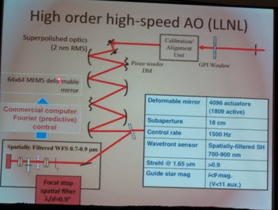 There are some interesting lessons they learned from the WFS:
 - small subapertures make it hard to align;
- mount of the camera is hard to align;
The controller they use is commercial closed black-box (Fourier, predictive controller).
The WFS used is Shack-Hartmann quadcell. WFS noise is 4-5 e- at 1 KHz speed.
The TMTracer: a modeling tool for the TMT alignment and phasing system, Piotr K. Piatrou, Gary A. Chanan, Univ. of California, Irvine (United States) . . . .[8149-03]
This is about the simulator of the TMT parts written by Piotr K. Piatrou on FORTRAN 95. No diffraction effects, only ray tracing.
This is for alignment and phase sensing of the telescope mirrors. The control of the wavefront is LS tomography - filtration of commands directly to DM. This is due to huge amount of data.
Athermal design of the optical tube assemblies for the ESO VLT Four Laser Guide Star Facility, Rens Henselmans, David Nijkerk, Martin Lemmen, Fred Kamphues, TNO Science and Industry (Netherlands) . . . .[8149-04]
Interesting speech about the design of LGS tube, they actually use it for VLT with 4 GS for lambda=589 nm and power 25 W.
Overview of the control strategies for the TMT alignment and phasing system, Piotr K. Piatrou, Gary A. Chanan, Univ. of California, Irvine (United States) . . . . . . . . .[8149-05]
The main goal here is to automatically control alignment of AO parts on the TMT. The multidirectional tomography is the mainstream approach for TMT alignment.The PAS (alignment and phasing system) is n open-loop system without accounting for the dynamics.
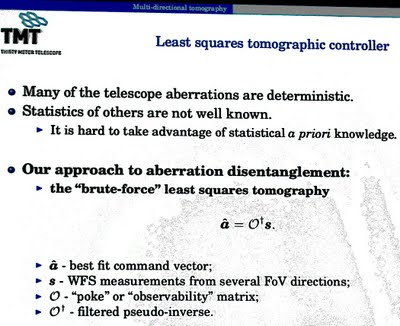
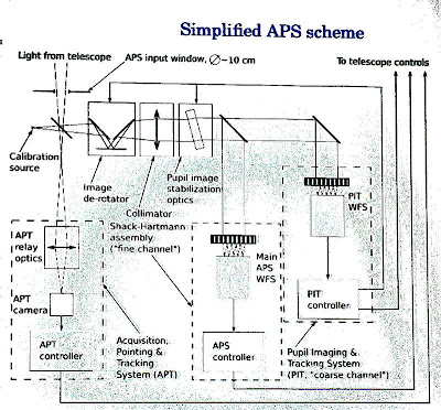 This is for the alignment only. The control is brute-force LS tomography because of huge amount of data. They have 33GB for SVD, and therefore use complexity reduction methods. For instance, projection mehtod like Oa = s -> \[ P\dagger O a = P\dagger a \]
 In the case of TMT, I think, it is possbile to nglect the dynamics of the system completely and just assume that the system is static. For low and medium frequencies it will probbly work well. That cruel algorithm (just throw the command to DM) explains the 2*opd coefficient 2.
The quasi-continuous part for the control.
Sunday, August 28, 2011
Manufacturing and using the continuous-facesheet deformable mirrors
It was interesting to know that Xinetics still uses very strong actuators that can actually break the mirror even in the presence of electrical protection. Some say they just do not want to upgrade their technology as NASA buys from them. Therefore, if there are very powerful actuators, the beackage of a mirror is possible. Other, like Gleb Vdovin from OKO Technologies, use soft actuators (piezoelectric ones) and the force of them is not enough to break the mirror.
How to attach an actuator to a Deformable Mirror?
Simple answer: using epoxy glue. Surprisingly, even after many days of work epoxy glue still holds actuators very well. Moreover, there were special tests: for instance, one can write a program (DMKILL) that throws random "0" and "+max" voltages on the mirror. It was reported that the first actuator broken down after at least 10 days (!) of constant work in such a regimen.
In the case of broken actuator, many people suggested just to throw it away as a loss of one actuator does not effects the rest too badly.
Main problem is Tip\Tilt
Tip and Tilt are the major sources of problems caused by the atmospheric turbulence. An impact of the higher aberrations falls very quickly. The correction is therefore required for the tip/tilt.
For this, a WFS with Zernike fitting can be helpful.
However, as Guan Ming Dai notes in his paper "Comparison of wavefront reconstructions with Zernike polynomials and Fourier transforms." [J Refract Surg. 2006 Nov;22(9):943-8.],
Fourier full reconstruction was more accurate than Zernike reconstruction from the 6th to the 10th orders for low-to-moderate noise levels. Fourier reconstruction was found to be approximately 100 times faster than Zernike reconstruction. Fourier reconstruction always makes optimal use of information. For Zernike reconstruction, however, the optimal number of orders must be chosen manually.
Wednesday, August 24, 2011
Interesting posters from SPIE Optical Engineering + Applications San Diego, CA, 2011
- Na variability and LGS elongation: impact on wavefront error, Katharine J. Jones, WBAO Consultant Group (United States). . . . . . . . . . . . . . . . . . . .[8149-14]
- MT_RAYOR: a versatile raytracing tool for x-ray telescopes, Niels Jørgen S.
Westergaard, Technical Univ. of Denmark (Denmark) . . . . . . . . . . . . . [8147-64] <---- this simulator is actually written on Yorick - A hardware implementation of nonlinear correlation filters, Saul Martinez-
Diaz, Hugo Castañeda Giron, Instituto Tecnológico de La Paz (Mexico)[8135-49] <--- the poster actually is about morphological filtres implemented in hardware. - Development of the visual encryption device using higher-order
birefringence, Hiroyuki Kowa, Takanori Murana, Kentaro Iwami, Norihiro
Umeda, Tokyo Univ. of Agriculture and Technology (Japan); Mitsuo Tsukiji,
Uniopt Co. Ltd. (Japan); Atsuo Takayanagi, Tokyo Univ. of Agriculture and
Technology (Japan) . . . . . . . . . . . . . . . . . . . . . . . . . . . . . . . . . . . . . . . . [8134-32] - Enhancement of the accuracy of the astronomical measurements carried
on the wide-field astronomical image data, Martin Rerábek, Petr Páta, Czech
Technical Univ. in Prague (Czech Republic) . . . . . . . . . . . . . . . . . . . . . [8135-58] - Astronomical telescope with holographic primary objective, Thomas D.
Ditto, 3DeWitt LLC (United States) . . . . . . . . . . . . . . . . . . . . . . . . . . . . [8146-40] - Calibration of the AVHRR near-infrared (0.86 μm) channel at the Dome
C site, Sirish Uprety, Changyong Cao, National Oceanic and Atmospheric
Administration (United States). . . . . . . . . . . . . . . . . . . . . . . . . . . . . . . . [8153-74]
Wednesday, August 17, 2011
A note about Greenwood frequency
where $v_w(z)$ is a wind velocity, and $\beta$ is the zenith angle. The Greenwood frequency can be associated with turbulence temporal error. The atmospheric turbulence conjugation process can be limited by temporal deficiencies as well as spatial ones\cite{karr1991temporal}. Assuming perfect spatial correction, Greenwood\cite{greenwoodbandwidth} showed that the variance of the corrected wavefront due to temporal limits is given by: $$\sigma^2_{temp} = \int_{0}^{\infty} |1 - H(f,f_c)|^2 P(f) df$$ where the $P(f)$ is the disturbance power spectrum\cite{tysonprinciplesbook}. The higher-order wavefront variance due to temporal constraints is $$\sigma_{temp}^2 = [\frac{f_G}{f_{3~dB}}]^{5/3}$$ where the $f_G$ is the Greenwood frequency.
Greenwood frequency as an estimation of a controller's bandwidth
The required frequency bandwidth of the control system is called the Greenwood frequency\cite{greenwoodbandwidth}. An adaptive optics system with a closed-loop servo response should reject most of the phase fluctuations. Greenwood\cite{greenwoodbandwidth} calculated the characteristic frequency $f_G$ as follows:
where $\beta$ is the zenith angle, $v_w$ is wind velocity. In the case of a constant wind and a single turbulent layer, the Greenwood frequency $f_G$ can be approximated by: $$f_G = 0.426 \frac{v_w}{r_0},$$ where $v_w$ as the velocity of the wind in meters/sec and $r_0$ is the Fried parameter. Greenwood\cite{greenwoodbandwidth} determined the required bandwidth, $f_G$ (the Greenwood frequency), for full correction by assuming a system in which the remaining aberrations were due to finite bandwidth of the control system\cite{saha2010aperture}. Greenwood derived the mean square residual wavefront error as a function of servo-loop bandwidth \textit{for a first order controller}, which is given by:
where $f_c$ is the frequency at which the variance of the residual wavefront error is half the variance of the input wavefront, known as 3 db closed-loop bandwidth of the wavefront compensator, and $f_G$ the required bandwidth\cite{saha2010aperture}. It must be noted that the required \textit{bandwidth for adaptive optics does not depend on height}, but instead is proportional to $v_w /r_0$ , which is in turn proportional to $\lambda^{-6/5}$. If the turbulent layer moves at a speed of 10 m/s, the closed loop bandwidth for $r_0 \approx 11$ cm, in the optical band (550 nm) is around 39 Hz\cite{saha2010aperture}.
For most cases of interest, the Greenwood frequency of the atmosphere is in the range of tens to hundreds of Hertz. Beland and Krause-Polstorff\cite{greenwoodfreqvariation} present measurements that show how the Greenwood frequency can vary between sites. Mt. Haleakala in Maui, Hawaii, has an average Greenwood frequency of 20 Hz. For strong winds and ultraviolet wavelengths, the Greenwood frequency can reach 600 Hz. The system bandwidth on bright guide stars is, in most cases, several times larger than the Greenwood frequency.
\begin{thebibliography}{1}

\bibitem{greenwoodbandwidth} D.~P. Greenwood.

\newblock Bandwidth specification for adaptive optics systems.

\newblock {\em J. Opt. Soc. Am.}, 67:390--93, 1977.


\bibitem{tysonprinciplesbook} R.~Tyson.

\newblock Principles of adaptive optics. \newblock 2010.


\bibitem{tyler1994bandwidth} G.A. Tyler.

\newblock Bandwidth considerations for tracking through turbulence.

\newblock {\em JOSA A}, 11(1):358--367, 1994.


\bibitem{karr1991temporal} T.J. Karr.

\newblock Temporal response of atmospheric turbulence compensation.

\newblock {\em Applied optics}, 30(4):363--364, 1991.


\bibitem{saha2010aperture} S.K. Saha.

\newblock Aperture synthesis: Methods and applications to optical astronomy.

\newblock 2010.


\bibitem{greenwoodfreqvariation} R.~Beland and J.~Krause-Polstorff.

\newblock Variation of greenwood frequency measurements under different   meteorological conditions.

\newblock In {\em Proc. Laser Guide Star Adaptive Optics Workshop 1, 289.   Albuquerque, NM: U. S. Air Force Phillips Laboratory}, 1992.

\end{thebibliography}
Monday, August 15, 2011
A laser from a living cell
 |
| From To Imaging, and Beyond! |
By the way, from the OPN journal again, the table of lasers and their power:

Quite nice.
Wednesday, August 3, 2011
Simulink tricks: multiple plots / two or more inputs on Scope
Trick 1: use Mux block
Use the Mux block from the Signal Routing palette:
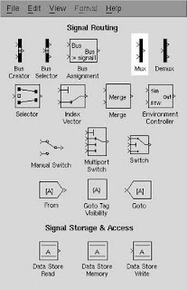
to merge two signals in one and connect them to Scope. Here is an example scheme:

Trick 2: use Vector concatenate block
Another solution is to use the Vector Concatenate block from the Signal Routing palette:
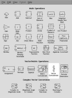
This trick will collect all the signals to be displayed, and then to connect the output from the vector concatenate block to the one input port of the Scope. In matrix case, of course, use Matrix concatenate. The example of schematics is presented below:

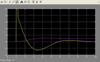
The result
Simulink will automatically highlight each signal by a different colour, as shown below:
Thursday, June 30, 2011
Books on Kalman Filter
Optimal State Estimate by Dan Simon
A very comprehensive book and, which is more important, it uses a bottom-up approach that enables readers to master the material rather quickly. Dan Simon's book is the best and the most suitable for self-study. Explanations are concise and straightforward. This book relates control theory elegantly. The author uses well laid out algorithmic approaches, suitable for programming, and examples to explain the details and show the complexities in action.
You will find all estimation topics in one book: Kalman filter, Unscented Kalman (UKF), Extended Kalman (EKF) and a very good explanation of Particle filtering (PF).
Moreover, the author has a website with a lot of MATLAB code for the examples used in book. This is a great help in terms of understanding of the subject, as most of examples are very insightful.
Introduction to Random Signals and Applied Kalman Filtering by Brown and Hwang
The book is easy to read and easy to follow: it starts from the very detailed explanation of the background needed for the Kalman filter. Obviously, the authors had an extensive teaching experience. The explanation of the Discrete Kalman Filter is one of the best I ever found. The extended KF and some implementation issues (UDU filter, sequential estimation) are not covered as well as other topics.
One should admit, however, that starting from the Chapter 6, the authors evidently exhausted and the text started to be more and more terse. The chapter about Kalman smoothing I could hardly translate to human language - better to use Dan Simon book.
Advanced Kalman Filtering, Least Squares and Modelling: A practical Handbook by Bruce Gibbs
The book is very terse in terms of explanations, and one should read it only as a reference, with a good background in Kalman filtering. Advanced topics, such as Particle Filter and Unscented Kalman, are covered in a very short manner and not very insightful. This is a handbook after all and not the book for the self-study. However, the book provides a lot of in-depth information and insight into various areas not found elsewhere.
This will be most useful for somebody with a strong mathematical background, particularly in linear algebra, who is looking for a comprehensive understanding and the best solution for a particular application.
Overall: a good reference, but not very helpful in terms of explanation.
Sunday, June 26, 2011
Notes on the structure of the scientific article
- abstract
- introduction
- methods (mathematical formulation)
- results
- discussion
- conclusion
- acknowledgements
Title
The title should be short and unambiguous, yet be an adequate description of the work. A general rule-of-thumb is that the title should contain the key words describing the work presented. Remember that the title becomes the basis for most on-line computer searches - if your title is insufficient, few people will find or read your paper.
Abstract
Once you have the completed abstract, check to make sure that the information in the abstract completely agrees with what is written in the paper. Confirm that all the information appearing the abstract actually appears in the body of the paper.
A well-prepared abstract enables the reader to identify the basic content of a document quickly and accurately. The abstract concisely states the principal objectives and scope of the investigation where these are not obvious from the title. The abstract must be concise; most journals specify a length, typically not exceeding 250 words. If you can convey the essential details of the paper in 100 words, do not use 200.
Introduction
The introduction defines the subject and must: outline the scientific objectives for the research performed and give the reader sufficient background to understand the rest of the report.
A good introduction will answer several questions:
1. Why was this study performed? Answers to this question may be derived from observations of nature or from the literature.
2. What knowledge already exists about this subject? That is review of the literature, showing the historical development of an idea and including the confirmations, conflicts, and gaps in existing knowledge.
3. What is the specific purpose of the study? The specific hypotheses and experimental design pertinent to investigating the topic should be described.
4. What is the Novelty of this paper? An important function of the introduction is to establish the significance of your current work: Why was there a need to conduct the study? Having introduced the pertinent literature and demonstrated the need for the current study, you should state clearly the scope and objectives.
Fundamental questions to answer here include:
- Do your results provide answers to your testable hypotheses? If so, how do you interpret your findings?
- Do your findings agree with what others have shown? If not, do they suggest an alternative explanation or perhaps a unforseen design flaw in your experiment (or theirs?)
- Given your conclusions, what is our new understanding of the problem you investigated and outlined in the Introduction?
- If warranted, what would be the next step in your study, e.g., what experiments would you do next?
Methods
Materials and methods used in the experiments should be reported. What equipment was used, what is the mathematics that describes the process?
However, it is still necessary to describe special pieces of equipment and the general theory of the assays used. This can usually be done in a short paragraph, possibly along with a drawing of the experimental apparatus.
Results
- All scientific names (genus and species) must be italicized. (Underlining indicates italics in a typed paper.)
- Use the metric system of measurements. Abbreviations of units are used without a following period.
- Be aware that the word data is plural while datum is singular. This affects the choice of a correct verb. The word species is used both as a singular and as a plural.
- Numbers should be written as numerals when they are greater than ten or when they are associated with measurements; for example, 6 mm or 2 g but two explanations of six factors. When one list includes numbers over and under ten, all numbers in the list may be expressed as numerals; for example, 17 sunfish, 13 bass, and 2 trout. Never start a sentence with numerals. Spell all numbers beginning sentences.
- Be sure to divide paragraphs correctly and to use starting and ending sentences that indicate the purpose of the paragraph. A report or a section of a report should not be one long paragraph.
- Every sentence must have a subject and a verb.
- Avoid using the first person, I or we, in writing. Keep your writing impersonal, in the third person. Instead of saying, "We weighed the frogs and put them in a glass jar," write, "The frogs were weighed and put in a glass jar."
- Avoid the use of slang and the overuse of contractions.
- Be consistent in the use of tense throughout a paragraph--do not switch between past and present. It is best to use past tense.
- Be sure that pronouns refer to antecedents. For example, in the statement, "Sometimes cecropia caterpillars are in cherry trees but they are hard to find," does "they" refer to caterpillars or trees?
Conclusion
Introductions and conclusions can be the most difficult parts of papers to write. While the body is often easier to write, it needs a frame around it. An introduction and conclusion frame your thoughts and bridge your ideas for the reader.
Your conclusion should make your readers glad they read your paper. Your conclusion gives your reader something to take away that will help them see things differently or appreciate your topic in personally relevant ways. It can suggest broader implications that will not only interest your reader, but also enrich your reader's life in some way.
Generally, three questions in the conclusion should be addressed:
1. What the problem was addressed?
2. What are results?
3. So what?
Play the "So What" Game. If you're stuck and feel like your conclusion isn't saying anything new or interesting, ask a friend to read it with you. Whenever you make a statement from your conclusion, ask the friend to say, "So what?" or "Why should anybody care?" Then ponder that question and answer it. Here's how it might go:
You: Basically, I'm just saying that education was important to Douglass.
Friend: So what?
You: Well, it was important because it was a key to him feeling like a free and equal citizen.
Friend: Why should anybody care?
You: That's important because plantation owners tried to keep slaves from being educated so that they could maintain control. When Douglass obtained an education, he undermined that control personally.
You can also use this strategy on your own, asking yourself "So What?" as you develop your ideas or your draft.
Synthesize, don't summarize. Include a brief summary of the paper's main points, but don't simply repeat things that were in your paper. Instead, show your reader how the points you made and the support and examples you used fit together.
Propose a course of action, a solution to an issue, or questions for further study. This can redirect your reader's thought process and help her to apply your info and ideas to her own life or to see the broader implications.
Looking to the future: Looking to the future can emphasize the importance of your paper or redirect the readers' thought process. It may help them apply the new information to their lives or see things more globally.
Monday, June 6, 2011
Books about Adaptive Optics
Adaptive Optics for Astronomical Telescopes (Oxford Series in Optical \& Imaging Sciences) by John Hardy
Hardy was a pioneer in adaptive optics and in the 1970s he built the first system capable of compensating the turbulence of a large astronomical telescope at visible wavelengths.
The book is very comprehensive, with an excellent bibliography and outstanding illustrations. The text is informative and consistent, with strong points in atmosphere turbulence and deformable mirrors. As a minor issues I must mention that the control part of adaptive optics is covered less deeply, but enough for the first-time reader. Despite of its age, the book gives all necessary background to enter to adaptive optics field.
The book by Hardy is by far The Best book in adaptive optics.
John W. Hardy, Adaptive optics for astronomical telescopes, Oxford University Press, USA, 1998.
Numerical Simulation of Optical Wave Propagation With Examples in MATLAB, by Jason Schmidt
The book presents the latest advances in numerical simulations of optical wave propagations in turbulent media. The book is clearly written and abundant of excellent examples in MATLAB giving to the reader a lot of step-by-step introductions as well as understanding of the waves propagation. The writing style is very engaging.
However, the Chapter 9 is slightly denser than others (I think it could be split on two different chapters). The operators notations used in Chapter 6 sometimes are more difficult to follow than conventional expressions. But those are minor issues that do not affect the material of the book.
Overall, the material of the book and the MATLAB code present a solid basis for the numerical simulations. Carefully selected bibliography of the book allows to use it as an excellent reference.
Jason D. Schmidt, Numerical Simulation of Optical Wave Propagation, With Examples in Matlab, Society of Photo-Optical Instrumentation Engineers, 2010.
Adaptive Optics in Astronomy by Francois Roddier
This is a very good example of how one should NOT write a book. This is not even a book but just a draft of several conference proceedings meshed together. There is no transition between chapters, the writing skills of different authors are very different and it is quite annoying.
For instance, in chapter about numerical simulations you will find NOTHING about how to really simulate the AO systems: no sinlge formula or plot. Chapter about ``theoretical'' background is written in a manner that there actually is a solid theory behind it - and most formulas are starting with numercial coefficient, which is improssible to get theoretically.
The second part of book is just a outdate garbage: stories of how the author built telescopes, with unnecessary detailed information that is useless now.
Don't waste your time on it.
Adaptive optics handbook by R.Tyson
The following books is by R. Tyson. Personally, I think that reading books from Tyson is mostly waste of time. He is like bakery that produces books as they are cakes. Very few useful information. More pity is that Tyson is a non-stop-backery than stamps and stamps books, one worse than other.
Monday, May 16, 2011
A note on Waffle Modes
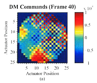
The commonly-used square Fried geometry[2] sensing in most Shack-Hartmann-based adaptive optics (AO) systems is insensitive to a checkerboard-like pattern of phase error called waffle. This zero mean slope phase error is low over one set of WFS sub-apertures arranged as the black squares of a checkerboard, and high over the white squares.
Waffle mode is essentially a repeated astigmatic pattern at the period of the SH sampling over the entire aperture. This wavefront has zero average slope over every sub-aperture and hence produces zero SH WFS output. The illustration of the waffle pattern on the DM is in Fig. 1.
Figure 1: Waffle mode on the DM [the picture from[3]]
Efforts have been made to understand how to control this and other ``blind'' reconstructor modes[1,4,5]. Advances in wave front reconstruction approaches have improved AO system performance considerably. Many physical processes cause the waffle: misregistration, high noise levels on the photosensor of WFS and so on.
Atmospheric turbulence and the Waffle modes
The initial uncertainty of atmospheric phase[1] is given by Kolmogorov statistics[6,7]. The atmosphere is unlikely to contain high spatial frequency components relative to low spatial frequency ones. Atmospheric turbulence has the form of a fractal and has much more power at large spatial scales so that the idea that the atmospheric wavefront can have big swings between adjacent phase points is physically unrealistic. This acts fortuitously to suppress waffle behaviour, which is a high spatial frequency behaviour.
Waffle modes during the Wavefront Sensing
The first step is to define the phase differences in terms of the phase measurements. Most gradient and curvature wavefront sensors do not sense all possible modes. For instance, the Fried geometry cannot measure the so-called Waffle mode. The Waffle mode occurs when the actuators are moved in a checkerboard pattern: all white squares change position while the black squares remain stationary. This pattern can build up over time, it is reduced by using different actuator geometries or filtering the control signals so as suppress this mode.The curvature WFS, is not sensitive to waffle mode error, although it has its own particular null space. Curvature sensors are typically not used for AO systems with more sensing channels because of their noise propagation properties[8].
We stress here that waffle mode error does not depend fundamentally on the actuator location and geometry: it only depends on the sensor geometry[9].
Waffle modes in Deformable Mirrors
The best DMs that we make use a quasi-hex geometry, which reduces waffle pattern noise. In the continuous-facesheet mirrors, the actuators push and pull on the surface. Since the surface in continuous, there is some mechanical crosstalk from one actuator to the next one - this is so-called influence function. But that can be controlled through software within the control computer. Because most DM have regular arrays of actuators, either square or hexagonal geometries, the alternate pushing and pulling of adjacent actuators can impart a patterned surface that resembles a waffle. The ``waffle mode'' can appear in images of regular patter, which acts an an unwanted diffraction grating[10].
Removing the waffle modes
There is a weighting approach proposed by Gavel[1] that will actually change the mode space structure. We introduce an actuator weighting, but instead of using a scalar regularisation parameter we use a positive-definite matrix. An a-priori statistical information concerning the quantities to be determined and the measurement noise can be used to set the weighting matrices in the cost function terms.The technique penalises all local waffle behaviour using the weighting matrix. It was found[1] that only a modification of the cost function by including a penalty term on the actuators will actually modify the mode space. With a suitable weighting matrix on the actuators, waffle behaviour can be sorted out into modes that have the least influence in the reconstruction matrix, thus suppressing waffle in the wavefront solutions.
The problem is that when the waffle modes go unsensed, they are not corrected by the DM and can accumulate within the closed-loop operation of the system. The accumulation of waffle modes leads to serious performance problems. The simplest way to correct them is that the adaptive-optics operator opens the feedback loop of the system in order to clear the DM commands and alleviate the waffle.
The waffle pattern accumulates in a closed-loop feedback system because the sensor cannot sense the mode for compensation. Spatially filtering the DM commands gives the option to maintain a conventional reconstructor while still having the ability to mitigate the waffle mode when it occurs[3]. In those experiments authors used a leaky integrator.
The paper[3] analyses a technique of sensing the waffle mode in the deformable mirror commands and applying a spatial filter to those commands in order to mitigate for the waffle mode. Directly spatially filtering the deformable mirror commands gives the benefit of maintaining the reconstruction of high frequency phase of interest while having the ability to alleviate for the waffle-like pattern when it arises[3].
This paper[3] will present a technique that only alleviates for the waffle when it is detected and does not effect the reconstruction of the phase when the mode has not accumulated to a degree that causes degradation in the performance of the system.
Bibliography
- 1
- D.T. Gavel.
Suppressing anomalous localized waffle behavior in least-squares wavefront reconstructors.
4839:972, 2003. - 2
- D.L. Fried.
Least-square fitting a wave-front distortion estimate to an array of phase-difference measurements.
JOSA, 67(3):370-375, 1977. - 3
- K.P. Vitayaudom, D.J. Sanchez, D.W. Oesch, P.R. Kelly, C.M. Tewksbury-Christle, and J.C. Smith.
Dynamic spatial filtering of deformable mirror commands for mitigation of the waffle mode.
In SPIE Optics & Photonics Conference, Advanced Wavefront Control: Methods, Devices, and Applications VII, Vol. 7466: 746609, 2009. - 4
- L.A. Poyneer.
Advanced techniques for Fourier transform wavefront reconstruction.
4839:1023, 2003. - 5
- R.B. Makidon, A. Sivaramakrishnan, L.C. Roberts Jr, B.R. Oppenheimer, and J.R. Graham.
Waffle mode error in the AEOS adaptive optics point-spread function.
4860:315, 2003. - 6
- A.N. Kolmogorov.
Dissipation of energy in the locally isotropic turbulence.
Proceedings: Mathematical and Physical Sciences, 434(1890):15-17, 1991. - 7
- A.N. Kolmogorov.
The local structure of turbulence in incompressible viscous fluid for very large Reynolds numbers.
Proceedings: Mathematical and Physical Sciences, 434(1890):9-13, 1991. - 8
- A. Glindemann, S. Hippler, T. Berkefeld, and W. Hackenberg.
Adaptive optics on large telescopes.
Experimental Astronomy, 10(1):5-47, 2000. - 9
- R. B. Makidon, A. Sivaramakrishnan, M. D. Perrin, L. C. Roberts, Jr., B. R. Oppenheimer, R. Soummer, and J. R. Graham.
An analysis of fundamental waffle mode in early aeos adaptive optics images.
The Publications of the Astronomical Society of the Pacific, 117:831-846, August 2005. - 10
- R.K. Tyson.
Adaptive optics engineering handbook.
CRC Press, 2000.
Monday, May 9, 2011
A note on speed comparison of wavefront reconstruction approaches
The reconstruction of the wavefront by means of the FFT was proposed by Freischlad and Koliopoulos\cite{freischlad1985wavefront} for square apertures on the Hudgin geometry. In a further paper\cite{FreischladFFTreconWFR} the authors derived methods for additional geometries, including the Fried geometry, which uses one Shack-Hartmann (SH) sensor. Freischlad also considered the case of small circular apertures\cite{freischladwfrfft} and the boundary problem was identified.
Computational speed comparison
The computational speed of Hudgin-FT and Fried-FT are limited only by the FFT\cite{poyneer2003advanced}. The extra processing to solve the boundary problem is of a lower order of growth computationally. Therefore FFT implementations have computational costs that scale as $O(n \log n)$. However, the implementation of Fried-FT requires potentially 2 times as much total computation as the Hudgin-FT. For the $64 \times 64$ grid, the FFT can be calculated on currently available systems in around 1 ms\cite{poyneer2003advanced}. If $N$ is a power of two the spatial filter, operations can be implemented with FFT's very efficiently. The computational requirements then scale as $O( N^2 log_2 N )$ rather than as $O( N^4 )$ in the direct vector-matrix multiplication approach. The modified Hudgin takes half as much computation as the Fried geometry model\cite{poyneer2003advanced}.
Comparison of FFT WFR and Zernike reconstruction speed
A very interesting paper appeared in the Journal of Refract Surgery\cite{dai2006comparison}. A comparison between Fourier and Zernike reconstructions was performed. In the paper\cite{dai2006comparison}, noise-free random wavefronts were simulated with up to the 15th order of Zernike polynomials. Fourier full reconstruction was more accurate than Zernike reconstruction from the 6th to the 10th orders for low-to-moderate noise levels. Fourier reconstruction was found to be approximately \textbf{100 times faster than Zernike reconstruction}. For Zernike reconstruction, however, the optimal number of orders must be chosen manually. The optimal Zernike order for Zernike reconstruction is lower for smaller pupils than larger pupils. The paper\cite{dai2006comparison} concludes that the FFT WFR is faster and more accurate than Zernike reconstruction, makes optimal use of slope information, and better represents ocular aberrations of highly aberrated eyes.
Noise propagation
Analysis and simulation show that for apertures just smaller than the square reconstruction grid (DFT case), the noise propagations of the FT methods are favourable. For the Hudgin geometry, the noise propagator grows with $O(\ln n)$. For the Fried geometry, the noise propagator is best-fit by a curve that is quadratic in the number of actuators, or $O(\ln^2 n)$. For fixed power-of-two sized grids (required to obtain the speed of the FFT for all aperture sizes) the noise propagator becomes worse when the aperture was much smaller than the grid\cite{poyneer2003advanced}.
Shack-Hartmann sensor gain
The Shack-Hartmann WFS produces a measurement which deviates from the exact wavefront slope. The exact shape of this curve depends on number of pixels used per sub-aperture and the centroid computation method (see \cite{hardyAObook} section 5.3.1 for a representative set of response curves). The most important feature of the response curve is that even within the linear response range, the gain of the sensor is not unity\cite{poyneer2003advanced}. This gain is important in the open-loop: in a closed loop this problem in mitigated by the overall control loop gain, which can be adjusted instead.
References:
\begin{thebibliography}{1} \bibitem{poyneer2003advanced} L.A. Poyneer. \newblock {Advanced techniques for Fourier transform wavefront reconstruction}. \newblock In {\em Proceedings of SPIE}, volume 4839, page 1023, 2003. \bibitem{PoyneerFastFFTreconWFR} Lisa~A. Poyneer, Donald~T. Gavel, and James~M. Brase. \newblock Fast wave-front reconstruction in large adaptive optics systems with use of the fourier transform. \newblock {\em J. Opt. Soc. Am. A}, 19(10):2100--2111, Oct 2002. \bibitem{freischlad1985wavefront} K.~Freischlad and C.L. Koliopoulos. \newblock {Wavefront reconstruction from noisy slope or difference data using the discrete Fourier transform}. \newblock 551:74--80, 1985. \bibitem{FreischladFFTreconWFR} Klaus~R. Freischlad and Chris~L. Koliopoulos. \newblock Modal estimation of a wave front from difference measurements using the discrete fourier transform. \newblock {\em J. Opt. Soc. Am. A}, 3(11):1852--1861, Nov 1986. \bibitem{freischladwfrfft} Klaus~R. Freischlad. \newblock Wave-front integration from difference data. \newblock {\em Interferometry: Techniques and Analysis}, 1755(1):212--218, 1993. \bibitem{dai2006comparison} G.~Dai. \newblock {Comparison of wavefront reconstructions with Zernike polynomials and Fourier transforms.} \newblock {\em Journal of refractive surgery}, 22(9):943--948, 2006. \bibitem{hardyAObook} John~W. Hardy. \newblock {\em {Adaptive optics for astronomical telescopes}}. \newblock Oxford University Press, USA, 1998. \end{thebibliography}
Monday, April 25, 2011
Reconstruction of the wavefront: Boundary problems on a circular aperture
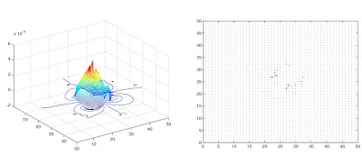 Reconstruction of the wavefront using FFT WFR modified Hudgin method is shown with the circular aperture and central obscuration (outer is 0.9, and inner is 0.1).
 In the case of astronomical telescopes, the gradients are typically available on
a circular aperture. The measurement data cannot be zero padded as it leads to large errors on boundaries. Such errors do not decrease with system size\cite{PoyneerFastFFTreconWFR}.
Because of the spatial periodicity and closed-path-loop conditions (see below), zero-padding the gradient measurements is incorrect. Doing so violates both conditions in general\cite{PoyneerFastFFTreconWFR}. These inconsistencies manifest themselves in errors that span the aperture. The errors do not become less significant as the aperture size increases: unlike the squareaperture case, the amplitude of the error remains large and spans the circular aperture.
Assumptions in the wavefront reconstruction that are not always true
There are two key assumptions in the wavefront reconstruction that must be satisfied for the proper work of the algorithm\cite{PoyneerFastFFTreconWFR}:
- the gradients are spatially periodic (necessary for use of the DFT method, and it must be maintained for a set of gradient measurements). Check if the sum of every row or column in the $N\times N$ gradient signal equals zero.
- any closed path of gradients must sum to zero (based on the modeling of the gradients as first differences).
- all loops (under Hudgin or Fried geometry) must sum to zero;
- both slope signals must be spatially periodic (for DFT)
The boundary problem is solved by using specific methods to make the gradient
sets consistent\cite{poyneer2003advanced}. These methods involve setting the values of specific gradients outside the aperture in a way to guarantee correct reconstruction inside the aperture. By using these methods FT reconstructors accurately reconstruct all sensed modes inside the aperture.
Solutions to the boundary problem: boundary method
The first method is the boundary method: it estimates the gradients that cross the boundary of the aperture\cite{PoyneerFastFFTreconWFR}. It follows directly from the development
above of inside, boundary, and outside gradients. Only the inside gradients are known from the measurement. The outside gradients can all be set to zero leaving the boundary gradients undetermined. A loop continuity equation can be written for each of the two smallest loops that involve a boundary gradient.
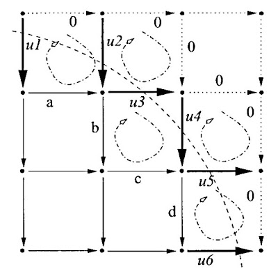 Boundary method. Setting each closed loop across the aperture edge to zero results in an equation relating the unknown boundary gradients to the measured inside gradients and the zeroed outside gradients [picture from the paper \cite{PoyneerFastFFTreconWFR}].
$\mathbf{M}u = c$
Here the matrix $M$ is specific for the selected geometry, the $u$ is the vector of all boundary gradients, and the $c$ is a vector containing sums of measured gradients (it has a fixed combination of gradients, but the value of these gradients depends on the actual measurement\cite{PoyneerFastFFTreconWFR}). In the case of noised measurements, the solution can be found using the pseudoinverse of the matrix $M$.
Solutions to the boundary problem: Extention method
The second method is the extension method: it extends out the gradients from inside the aperture. The extension method extends the wavefront shape to
outside the aperture. It does this by a preserving loop continuity\cite{PoyneerFastFFTreconWFR}. The x gradients are extended up and down out of the aperture, while the y gradients are extended to the left and the right.
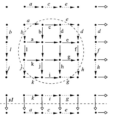
The extension method produces a completely consistent set of gradients. These provide perfect reconstruction of the phase when there is no noise, except for the piston. If there is noise, the same procedure is done, though loop continuity will not hold on loops involving the seam gradients, just as the boundary gradients in the boundary method were the best, but not an exact, solution when there was noise\cite{PoyneerFastFFTreconWFR}.
References:
\begin{thebibliography}{1}
\bibitem{PoyneerFastFFTreconWFR} Lisa~A. Poyneer, Donald~T. Gavel, and James~M. Brase. \newblock Fast wave-front reconstruction in large adaptive optics systems with use of the fourier transform. \newblock {\em J. Opt. Soc. Am. A}, 19(10):2100--2111, Oct 2002.
\bibitem{poyneer2003advanced} L.A. Poyneer. \newblock {Advanced techniques for Fourier transform wavefront reconstruction}. \newblock In {\em Proceedings of SPIE}, volume 4839, page 1023, 2003.
\end{thebibliography}
Monday, April 18, 2011
Simple model of ADC, noises in ADC and ADC non-linearity
An ADC has an analogue reference voltage $V_{REF}$ or current against which the analogue input is compared. The digital output tells us what fraction of the reference voltage or current is the input voltage or current. So if we have N-bit ADC, there are $2^N$ possible output codes, and the difference between each output code is $\frac{V_{REF}}{2^N}$.
Resolution of ADC
Every time you increase the input voltage by $V_{REF}/2^N$ Volt, the output code will increase by one bit. This means that the least significant bit (LSB) represents $V_{REF}/2^N$ Volt, which is the smallest increment that the ADC actually can \textit{resolve}. Then one can say that the \textit{resolution} of this converter is $V_{REF}/2^N$ because ADC resolve voltages as small as such value. Resolution may also be stated in bits.
Because the resolution is $V_{REF}/2^N$, better accuracy / lower error can be achieved as: 1) use a higher resolution ADC and/or 2) use a smaller reference voltage. The problem with high-resolution ADC is the cost. Moreover, the higher resolution / lower $V_{REF}/2^N$, the more difficult to detect a small signal as it becomes lost in the noise thus reducing SNR performance of the ADC. The problem with reducing $V_{REF}$ is a loss of input dynamic range.
Hence the ADC's resolution indicates the number of discrete values that can be produced over the range of analogueue values and can be expressed as:
$$ K_{ADC} = (V_ \mathrm {REF} - V_ \mathrm {min})/N_{max}$$
where $V_ \mathrm {REF}$ is maximum (reference) voltage that can be quantified, $V_ \mathrm {min}$ is minimum quantifiable voltage, and $N_{max} = 2^M$ is the number of voltage intervals ($M$ is ADC's resolution in bits). The ADC's output code can be represented as:
$$ADC_ \mathrm {Code} = \textrm{round}\left[ (V_ \mathrm {input}-V_ \mathrm {min})/K_{ADC} \right]$$
The lower reference voltage $V_{REF}$, the smaller range of voltages with greater accuracy one can measure. This is a common way to get better precision from an ADC without buying a more expensive ADC with higher resolution.
Quantisation error
As the input voltage in ADC increases towards $V_{REF}/2^N$, the output still remains at zero because a range of input voltages is represented by a single output code. When the input reaches $V_{REF}/2^N$, the output code changes from 000 to 001.
The maximum error in ADC is 1 LSB. This 0 to 1 LSB range is known as the ``quantisation
uncertainty'': there is a range of analogue input values that could have caused any given code.
Linearity and Linearity errors
The accuracy of analogue to digital conversion has an impact on overall system quality and efficiency. To be able to improve accuracy you need to understand the errors associated with the
ADC and the parameters affecting them.
Differential Linearity Error
Differential Linearity Error (DLE) describes the error in step size of an ADC: it is the maximum deviation between actual steps and the ideal steps (code width). Here ``ideal steps''' are not for the ideal transfer curve but for the resolution of the ADC. The input code width is the range of input values that produces the same digital output code.
Ideally analogue input voltage change of 1 LSB should cause a change in the digital code. If an analogue input voltage greater than 1 LSB is required for a change in digital code, then the ADC has the differential linearity error.
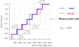
Here each input step should be precisely 1/8 of reference voltage. The first code transition from 000 to 001 is caused by an input change of 1 LSB as it should be. The second transition, from 001 to 010, has an input change that is 1.2 LSB, so is too large by 0.2 LSB. The input change for the third transition is exactly the right size. The digital output remains
constant when the input voltage changes from 4 LSB to 5 LSB, therefore the code 101
can never appear at the output.
When no value of input voltage will produce a given output code, that code is missing from the ADC transfer function. In data sheets of many ADC it is specified ``no missing codes''; this can be critical in some applications like servo systems.
Integral Linearity Error
Integral Linearity Error (ILE) describes the maximum deviation of ADC transfer function from a linear transfer curve (i.e. between two points along the input-output transfer curve). It is a measure of the straightness of the transfer function and can be greater than the differential non-linearity. In specifications, an ADC is described sometimes as being ``x bits linear.''
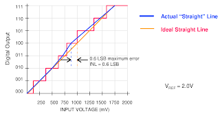
The ADC input is usually connected to an operational amplifier, maybe a summing or a differential amplifier which are linear circuits and process an analogue signal. As the ADC is included in the signal chain, we would like the same linearity to be maintained at the ADC level as well. However, inherent technological limitations make the ADC non-linear to some extent and this is where the ILE comes into play.
For each voltage in the ADC input there is a corresponding word at the ADC output. If an ADC is ideal, the steps are perfectly superimposed on a line. But most of real ADC exhibit deviation from the straight line, which can be expressed in percentage of the reference voltage or in LSBs.
The ILE is important because it cannot be calibrated out. Moreover, the ADC non-linearity is often unpredictable: it is difficult to say where on the ADC scale the maximum deviation from the ideal line is. Let's say the electronic device we design has an ADC that needs to measure the input signal with a precision of $\alpha$\% of reference voltage. Due to the ADC quantisation, if we choose a N-bit ADC, the initial measurement error is $E_{ADC} = \pm 0.5$ LSB, which is called the quantisation error:
$$ADC_{qantiz.error} = E_{ADC}/2^N $$
For instance, with 12-bit ADC and measurement error $\pm 1/2$ LSB, quantisation error will be $ADC_{qantiz.error} = \frac{1}{2 \cdot 2^{12}} \approx 0.0012 \% $. If we need to measure the input signal with precision of 0.1\% of VREF, 12-bit ADC does a good job. However, if the INL is large, the actual ADC error may come close to the design requirements of 0.5\%.
Signal-to-Noise ratio for ADC
Signal-to-Noise Ratio (SNR) is the ratio of the output signal amplitude to the output noise level. SNR of ADC usually degrades as frequency increases because the accuracy of the comparator(s) within the ADC degrades at higher input slew rates. This loss of accuracy shows up as noise at the ADC output.
Noise in an ADC comes from four sources:
- quantisation noise;
- noise generated by the ADC itself;
- application circuit noise;
- jitter;
The non-linearity of the ADC can be described as input to output transfer function of:
$Output = Input^{\alpha}$
Quantisation noise
Quantisation noise results from the quantisation process - the process of assigning an output code to a range of input values. The amplitude of the quantisation noise decreases as resolution increases because the size of an LSB is smaller at higher resolutions, which reduces the maximum quantisation error. The theoretical maximum of SNR for an ADC with a full-scale sine-wave input derives from quantisation noise
and is about $6.02\cdot N + 1.76$ dB.
Noise generated by the ADC itself
The problem can be in high capacitance of ADC output or input. Device input capacitances causes noise on the supply line. Discharging these capacitances adds noise to the ADC substrate and
supply bus, which can appear at the input as noise.
Minimising the load capacitance at the output will minimise the currents needed to charge and
discharge them, lowering the noise produced by the converter itself. This implies that one
output pin should drive only one input device pin (use a fan-out of one) and the length of the
ADC output lines should be as short as possible.
Application circuit noise
Application circuit noise is that noise seen by the converter as a result of the way the circuit is designed and laid out, for instance, noisy components or circuitry: noisy amplifiers, noise in resisters.
Amplifier noise is an obvious source of noise, but it is extremely difficult to find an amplifier with noise and distortion performance that will not degrade the system noise performance with a high resolution (12-bit or higher) ADC.
We often think of resistors as noisy devices, but choosing resistor values that are as low as
practical can keep noise to a level where system performance is not compromised.
Jitter
A clock signal that has cycle-to-cycle variation in its duty cycle is said to exhibit jitter. Clock jitter causes an uncertainty in the precise sampling time, resulting in a reduction of dynamic performance.
Jitter can result from the use of a poor clock source, poor layout and grounding. One can see that the steps of digital signal in case of jitter are rough and non-uniform.
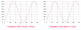
SNR performance decreases at higher frequencies because the effects of jitter get worse.
Types of ADC
There are different type of ADC schemes, each of them has own advantages and disadvantages.
For example, a Flash ADC has drifts and uncertainties associated with the comparator levels, which lead to poor uniformity in channel width and therefore poor linearity.
Poor linearity is also apparent for SAR ADCs, however it is less than that of flash ADCs. Non-linearity in SAR ADC arises from accumulating errors from the subtraction processes.
Wilkinson ADCs can be characterised as most linear ones; particularly, Wilkinson ADCs have the best (smallest) differential non-linearity.
Flash (parallel encoder) ADC
Flash ADCs are made by cascading high-speed comparators. For an N-bit ADC, the circuit employs 2N-1 comparators. A resistive-divider with 2N resistors provides the reference voltage. The reference voltage for each comparator is one least significant bit (LSB) greater than the reference voltage for the comparator. Each comparator produces a 1 when its analogue input voltage is higher than the reference voltage applied to it. Otherwise, the comparator output is 0.
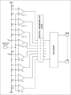 [the Image from the reference, (c) Maxim-ic]
The key advantage of this architecture is very fast conversion times, which is suitable for high-speed low-resolution applications.
The main disadvantage is its high power consumption. The Flash ADC architecture becomes prohibitively expensive for higher resolutions. [the reference used, (c) Maxim-ic]
Successive approximation register ADC
Successive-approximation-register (SAR) ADCs are the majority of the ADC market for medium- and high-resolution. SAR ADCs provide up to 5Msps sampling rates with resolutions from 8 to 18 bits. The SAR architecture allows for high-performance, low-power ADCs to be packaged in small form factors. The basic architecture is shown in Fig.~\ref{fig:SARADC}.
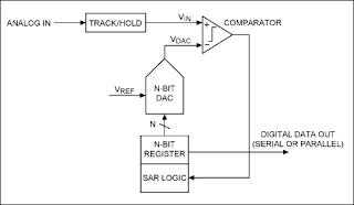 [ the Image from this reference, (c) Maxim-ic]
The analogue input voltage (VIN) is held on a track/hold. To implement the binary search algorithm, the N-bit register is first set to midscale. This forces the DAC output (VDAC) to be VREF/2, where VREF is the reference voltage provided to the ADC.
A comparison is then performed to determine if VIN is less than, or greater than, VDAC. If VIN is greater than VDAC, the comparator output is a logic high, or 1, and the MSB of the N-bit register remains at 1. Conversely, if VIN is less than VDAC, the comparator output is a logic low and the MSB of the register is cleared to logic 0.
The SAR control logic then moves to the next bit down, forces that bit high, and does another comparison. The sequence continues all the way down to the LSB. Once this is done, the conversion is complete and the N-bit digital word is available in the register.
Generally speaking, an N-bit SAR ADC will require N comparison periods and will not be ready for the next conversion until the current one is complete. This explains why these ADCs are power- and space-efficient. Another advantage is that power dissipation scales with the sample rate.[the reference used, (c) Maxim-ic]


