Compressed sensing: notes and remarks

This short note is about the tutorial [1] on compressed sensing (CS) recently published in Optical Engineering journal. The tutorial introduces a mathematical framework that provide insight into how a high resolution image can be inferred from a relatively small number of measurements. Among other applications, such as IR imaging and compressing video sequences, astronomical applications [2] of CS are very attractive.


The idea of Compressed Sensing
The basic idea of CS [1] is that when the image of interest is very sparse or highly compressible in some basis, relatively few well-chosen observations suffice to reconstruct the most significant nonzero components. It can be also considered as projecting onto incoherent measurement ensembles [2]. Such an approach should be directly applied in the design of the detector. Devising an optical system that directly “measures” incoherent projections of the input image would provide a compression system that encodes in the analog domain.

Rather than measuring each pixel and then computing a compressed representation, CS suggests that we can measure a “compressed” representation directly.

The paper [1] provides a very illustrative example of searching the bright dot on a black background: instead of full comparison (N possible locations), the CS allows to do it in M=log2(N) binary measurements using binary masks.

The picture from the paper [1]

The key insight of CS is that, with slightly more than K well-chosen measurements, we can determine which coefficients of some basis are significant and accurately estimate their values.

A hardware example of Compressed sensing
An example of a CS imager is the rice single-pixel camera developed by Duarte et al [3,4]. This architecture uses only a single detector element to image a scene. A digital micromirror array is used to represent a pseudorandom binary array, and the scene of interest is then projected onto that array before the aggregate intensity of the projection is measured with a single detector.


Using Compressed Sensing in Astronomy
Astronomical images in many ways represent a good example of highly compressible data. An example provided in [2] is Joint Recovery of Multiple Observations. In [2], they considered a case that the data are made of N=100 images such that each image is a noise-less observation of the same sky area. The goal is to propose the decompression the set of observations in a joint recovery scheme. As the paper [2] shows, CS provides better visual and quantitative results: the recover SNR for CS is 46.8 dB, while for the JPEG2000 it is only 9.77 dB.

Remarks on using the Compressed Sensing in Adaptive optics
The possible application of the CS in AO can be for centroiding estimation. Indeed, the centroid image occupies only a small portion of the sensor. The multiple observations of the same centroid can lead to increased resolution in centroiding and, therefore, better overall performance of the AO system.

References:
[1] Rebecca M. Willett, Roummel F. Marcia, Jonathan M. Nichols, Compressed sensing for practical optical imaging systems: a tutorial. Optical Engineering 50(7), 072601 (July 2011).

[2] Jérôme Bobin, Jean-Luc Starck, and Roland Ottensamer, Compressed Sensing in Astronomy, IEEE JOURNAL OF SELECTED TOPICS IN SIGNAL PROCESSING, VOL. 2, NO. 5, OCTOBER 2008.

[3] M. F. Duarte, M. A. Davenport, D. Takhar, J. N. Laska, T. Sun, K. Kelly, and R. G. Baraniuk, “Single-pixel imaging via compressive sampling,” IEEE Signal Process. Mag. 25(2), 83–91 (2008).

[4] W. L. Chan, K. Charan, D. Takhar, K. F. Kelly, R. G. Baraniuk, and D. M. Mittleman, “A single-pixel terahertz imaging system based on compressed sensing,” Appl. Phys. Lett. 93, 121105 (2008).

Nip2 - the advanced images analysis tool

The nip2 is a unique images analysis tool - it is not a conventional graphical editor like Adobe Photoshop or The GIMP.

The nip2 approach: each processing result is a cell
Nip2 has a non-trivial yet productive interface that is a kind of mix between a spreadsheet and a graphical editor (imagine a cocktail with Photoshop and Excel). The result of any operation is put down into a cell and you can make references to any cell (that is an image after some processing operation). For example, you can select the area of interest (cell A2) on the original image (cell A1) and apply some filter to region of interest that will be A3 cell. Such an interface allows you to quickly recalculate the resulting image if any parameters of previous filters have been changed.
The screenshot illustrates such paradigm.


Hence the nip2 is not a conventional graphical editor but rather a graphical analyser. Nip2 supports the most useful graphical formats such as TIFF, JPEG, PNG, PPM, as well as scientific formats like MAT (MATLAB's matrices) and convolution matrices. Thanks for using VIPS library, the nip2 allows to view extremely large images very fast: you definitely appreciate such feature is you process scientific data.

What is expected to find in NIP2 and what is not
To reiterate, the nip2 is rather a scientific images analysis laboratory than just another raster images editor. So there are no tools for layers and masking (and such tools are not needed). But when one deals with large images such as panorama, nip2 is priceless. Moreover, there are many advanced images processing algorithms that are hardly to be found in conventional editors: morphological images analysis, Fourier transform, statistical tools, and many other.

Few words about the interface of nip2
As above, the spreadsheet-like paradigm of nip2's interface allows you to change filter's parameters and quickly recalculate the resulting image. I'm going to show this on an example.
For instance, there is a sequence of filters that you need to apply on image - changing one parameter results on the destination image. Then you need to apply the filtering sequence for another image - and here the nip2 to rescue you: just right-click on any cell in nip2 and select "Replace from file".
That is enough for recalculation of the whole filtering sequence.


Intensity-scale change for images viewing
This is a very helpful feature when you need to view an image with specific grey levels (e.g., 12-bit raw images from the digital camera).

In order to change the intensity scale of the image, just left-drag to set number of brightness or contrast magnification. It does not affect on the real image's values but just for viewing.


Quick zooming
If you need to zoom-in or out quickly, just hold CTRL button on the keyboard and turn mouse's wheel.


Hotkeys in в nip2
The assignment of the hotkey for any menu function is really easy: just open nip2's menu, select the item and (when the item is selected) press a hotkey combination. The hotkey combination for that function will be assigned instantly.


Fast region selection
If you need to select the region of interest on the image, just hold CTRL keyboard button and start selecting the area on the image. A new cell that contains the selected appears instantly in the current column and the next number (e.g., if the current column is B and the last number of cell is 14, cell B15 with the region appears).


Quick scrolling of the image
Use the wheel, Luke! When viewing the image in the window, one can scroll the image up-down using mouse wheel. Moreover, holding SHIFT button and scrolling moves viewing area left and right, so you can completely neglect scrollbars.


Images analysis in nip2
Using nip2, one can perform advanced images processing and analysis by such tools as Fourier transform, correlation analysis, filtering and morphological analysis. The most common examples that I use daily have been provided below.

Fourier analysis in nip2
In many cases it is necessary to look not only on the image but on its Fourier spectrum. In contrast with conventional images editors, there are no problems in nip2: just use Toolkits - Math - Fourier - Forward and enjoy. You should nonetheless take into account that for large images Fourier transform can take a long time (~10-15 seconds depends on CPU's horsepower).

The reverse Fourier can be performed likewise using Toolkits - Math - Fourier - Reverse .


Images' histograms in nip2
A histogram can deliver the information about how much pixels of the same level contains the image being analysed. Indeed, this is a very useful feature, and you can find it in Toolkits - Histogram - Find - One Dimension.

As a result, we have a beautiful and informative histogram for the image.


Images edition in nip2
Of course you can edit and transform images in nip2 but some of the functions can look like kind a philosophical.

Cropping
There are two ways to crop the image: use Toolkits - Image - Crop or just open the cell with the image and select the region of interest.

Or, using menu one can select the region of interest likewise: File - New - New Region.


After that, you can save the cropped image by right-click and select "Save image as".


Threshold
The threshold function is concealed in the menu in Toolkits - Image - Select - Threshold.

Joining images in nip2
One of the most exciting feature of nip2 is joining images. While Photoshopers and Gimpers are buying heaps of RAM for their computers, nip2 users can join large images easily. Just use Toolkits - Image - Join - Left to Right or Toolkits - Image - Join - Top to Bottom and what we have:

This is much more easy and way faster than in Photoshop or Gimp: I have glued together 10x10 images each of which is 3000x2000 pixels on a notebook computer with only 512Mb RAM.


Tilt brightness
It happens sometime, and brightness tilt is very boring effect (i.e., when you analysing images from microscope, it is difficult to capture it without such brightness artefacts). But using nip2, one can correct tilt brightness using Tools - Filters - Tilt brightness.
Such function restores correct illumination on the image (to some extent, of course).

Conclusion
This post is actually a collection of my favorite tips and tricks of work in nip2. I'm going to update this post from time to time. And, of course, I would like to thank John Cupitt, Kirk Martinez, and Joe Padfield for such a great program!

Small survey of Objective Image Quality metrics

PDF version of this post is here

The importance of objective quality metric methods cannot be underestimated: such methods are being used in automated images restoration algorithms, for comparison of images compression algorithms and so on. Quality metrics are graphically presented in Fig. 1.

All proposed quality metrics can divided to two general classes¹: subjective and objective [2].

Subjective evaluation of images quality is oriented on Human Vision System (HVS). As it was mentioned in [3], the best way to assess the quality of an image is perhaps to look at it because human eyes are the ultimate receivers in most image processing environments. The subjective quality measurement Mean Opinion Score (MOS) has been used for many years.

Objective metrics include Mean Squared Error (MSE), or $L_p$-norm [4,5], and measures that are mimicking the HVS such as [6,7,8,9,10,11]. In particular, it is well known that a large number of neurons in the primary visual cortex are tuned to visual stimuli with specific spatial locations, frequencies, and orientations. Images quality metrics that incorporate perceptual quality measures by considering human visual system (HVS) were proposed in [12,13,14,15,16]. Image quality measure (IQM) that computes image quality based on the 2-D spatial frequency power spectrum of an image was proposed in [10]. But still such metrics have poor performance in real applications and widely criticized for not correlating well with perceived quality measurement [3].

As a promising techniques for images quality measure, Universal Quality Index [17,3], Structural SIMilarity index [18,19], and Multidimensional Quality Measure Using SVD [1] are worth to be mentioned ².

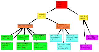
Figure 1: Types of images quality metrics.

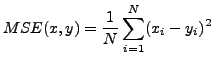
So there are three objective methods of images' quality estimation to be discussed below: the UQI, the SSIM, and MQMuSVD. Brief information about main ideas of those metrics is given. But first of all, let me render homage to a mean squared error (MSE) metric.

A Good-Old MSE

Considering that $x={x_i | i = 1,2,\dots N}$ and $y={x_i | i = 1,2,\dots N}$ are two images, where N is the number of image's pixels, the MSE between these images is:
Of course, there is more general and well-suitable formulation of MSE for images processing given by Fienup [5]:

(2)

where

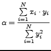(3)

Such NRMSE metrics allows to estimate quality of images especially in various applications of digital deconvolution techniques. Although Eq. 2 is better than pure MSE, the NRMSE metric have been criticizing a lot.

As it was written in remarkable paper [19], the MSE is used commonly for many reasons. The MSE is simple, parameter-free, and easy to compute. Moreover, the MSE has clear physical meaning as the energy of the error signal. Such an energy measure is preserved after any orthogonal linear transformation, such as Fourier transform. The MSE is widely used in optimization tasks and in deconvolution problem [21,22,23]. Finally, competing algorithms have most often been compared using the MSE or Peak SNR ratio.

But problems arising when one is trying to predict human perception of image fidelity and quality using MSE. As it was shown in [19], the MSE is very similar despite the differences in image's distortions. That is why there were many attempts to overcome MSE's limitations and find a new images quality metrics. Some of them are briefly discussed below.

Multidimensional Quality Measure Using SVD

The new metric of images quality called ``Multidimensional Quality Measure Using SVD'' was proposed in [1]. The main idea is that every real matrix A can be decomposed into a product of 3 matrices A = USV<sup>T</sup>, where U and V are orthogonal matrices, U<sup>T</sup>U = I, V<sup>T</sup>V = I, and $S = diag (s_1, s_2, \dots)$. The diagonal entries of S are called the singular values of A, the columns of U are called the left singular vectors of A, and the columns of V are called the right singular vectors of A. This decomposition is known as the Singular Value Decomposition (SVD) of A [24]. If the SVD is applied to the full images, we obtain a global measure whereas if a smaller block is used, we compute the local error in that block:
$s_i$ are the singular values of the original block, $\hat{s}_i$ are the singular values of the distorted block, and N is the block size. If the image size is $K$, we have $(K/N) \times (K/N)$ blocks. The set of distances, when displayed in a graph, represents a ``distortion map''.

A universal image quality index (UQI)

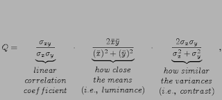
As a more promising new paradigm of images quality measurements, a universal image quality index was proposed in [17]. This images quality metric is based on the following idea:

The main function of the human eyes is to extract structural information from the viewing field, and the human visual system is highly adapted for this purpose. Therefore, a measurement of structural distortion should be a good approximation of perceived image distortion.

The key point of the new philosophy is the switch from error measurement to structural distortion measurement. So the problem is how to define and quantify structural distortions. First, let's define a necessary mathematics [17] for original image X and test image Y . The universal quality index can be written as [3]:

(5)

where

The first component is the linear correlation coefficient between x and y, i.e., this is a measure of loss of correlation. The second component measures how close the mean values are between x and y, i.e., luminance distortion. The third component measures how similar the variances of the signals are, i.e., contrast distortion.

UQI quality measurement method is applied to local regions using sliding window approach. For overall quality index to be obtained, average value of local quality indexes $Q_i$ must be calculated:

(6)

As it mentioned in [17], the average quality index UQI coincides with the mean subjective ranks of observers. That gives to researchers a very powerful tool for images' quality estimation.

Structural SIMilarity (SSIM) index

The Structural Similarity index (SSIM) that is proposed in [18] is a generalized form of a Universal Quality Index [17]. As above, $x$ and $y$ are discrete non-negative signals; $\mu_x$, $\sigma_{x}^2$, and $\sigma_{xy}$ are the mean value of $x$, the variance of $x$, and the covariance of $x$ and $y$, respectively. According to [18] the luminance, contrast, and structure comparison measures were given as follows:

			(7)
			(8)
			(9)

where $C_1$, $C_2$ and $C_3$ are small constants given by $C_1 = (K_1\cdot L)^2$ ; $C_2 = (K_2 \cdot L)^2$ and $C_3 = C_2/2$. Here $L$ is the dynamic range of the pixel values, and $K_1 \ll 1$ and $K_2 \ll 1$ are two scalar constants. The general form of the Structural SIMilarity (SSIM) index between signal x and y is defined as:

(10)

where $\alpha, \beta, \; \text{and} \; \gamma$ are parameters to define the relative importance of the three components [18]. If $\alpha= \beta= \gamma =1$, the resulting SSIM index is given by:

(11)

SSIM is maximal when two images are coinciding (i.e., SSIM is <=1 ). The universal image quality index proposed in [17] corresponds to the case of $C_1 = C_2 = 0$ , therefore is a special case of Eq. (11).

A drawback of the basic SSIM index is its sensitivity to relative translations, scalings and rotations of images [18]. To handle such situations, a waveletdomain version of SSIM, called the complex wavelet SSIM (CW-SSIM) index was developed [25]. The CWSSIM index is also inspired by the fact that local phase contains more structural information than magnitude in natural images [26], while rigid translations of image structures leads to consistent phase shifts.

Despite its simplicity, the SSIM index performs remarkably well [18] across a wide variety of image and distortion types as has been shown in intensive human studies [27].

Instead of conclusion

As it was said in [18], ``we hope to inspire signal processing engineers to rethink whether the MSE is truly the criterion of choice in their own theories and applications, and whether it is time to look for alternatives.'' And I think that such articles provide a great deal of precious information for making decision to give away the MSE.


Useful links:
A very good and brief survey of images quality metrics, with links to MATLAB examples. Zhou Wang's page with huge amount of articles and MATLAB source code for UQI and SSIM. Another useful link for HDR images quality metrics.

Bibliography

1

Aleksandr Shnayderman, Alexander Gusev, and Ahmet M. Eskicioglu.
A multidimensional image quality measure using singular value decomposition.
In Image Quality and System Performance. Edited by Miyake, Yoichi; Rasmussen, D. Rene. Proceedings of the SPIE, Volume 5294, pp. 82-92, 2003.

2

A. M. Eskicioglu and P. S. Fisher.
A survey of image quality measures for gray scale image compression.
In Proceedings of 1993 Space and Earth Science Data Compression Workshop, pp. 49-61, Snowbird, UT, April 2, 1993.

3

Ligang Lu Zhou Wang, Alan C. Bovik.
Why is image quality assessment so difficult?
In In: Proceedings of the ICASSP'02, vol. 4, pp. IV-3313-IV-3316., 2002.

4

W. K. Pratt.
Digital Image Processing.
John Wiley and Sons, Inc., USA, 1978.

5

J.R. Fienup.
Invariant error metrics for image reconstruction.
Applied Optics, No 32, 36:8352-57, 1997.

6

J. L. Mannos and D. J. Sakrison.
The effects of a visual fidelity criterion on the encoding of images,.
IEEE Transactions on Information Theory, Vol. 20, No. 4:525-536, July 1974.

7

J. O. Limb.
Distortion criteria of the human viewer.
IEEE Transactions on Systems, Man, and Cybernetics, Vol. 9, No. 12:778-793, December 1979.

8

H. Marmolin.
Subjective mse measures.
IEEE Transactions on Systems, Man, and Cybernetics, Vol. 16, No. 3:486-489, May/June 1986.

9

J. A. Saghri, P. S. Cheatham, and A. Habibi.
Image quality measure based on a human visual system model.
Optical Engineering, Vol. 28, No. 7:813-818, July 1989.

10

B. N. Norman and H. B. Brian.
Objective image quality measure derived from digital image power spectra.
Optical Engineering, 31(4):813-825, 1992.

11

A.A. Webster, C. T. Jones, M. H. Pinson, S. D. Voran, and S. Wolf.
An objective video quality assessment system based on human perception.
In Proceedings of SPIE, Vol. 1913, 1993.

12

T. N. Pappas and R. J. Safranek.
in book ``Handbook of Image and Video Processing'' (A.Bovik, ed.), chapter Perceptual criteria for image quality evaluation.
Academic Press, May 2000.

13

B. Girod.
in book Digital Images and Human Vision (A. B. Watson, ed.), chapter What's wrong with mean-squared error, pages 207-220.
the MIT press, 1993.

14

S. Daly.
The visible difference predictor: An algorithm for the assessment of image fidelity.
In in Proceedings of SPIE, vol. 1616, pp. 2-15, 1992.

15

A. B. Watson, J. Hu, and J. F. III. McGowan.
Digital video quality metric based on human vision.
Journal of Electronic Imaging, vol. 10, no. 1:20-29, 2001.

16

J.-B. Martens and L. Meesters.
Image dissimilarity.
Signal Processing, vol. 70:155-176, Nov. 1998.

17

Z. Wang and A.C. Bovik.
A universal image quality index.
IEEE Signal Processing Letters, vol. 9, no. 3:81-84, Mar. 2002.

18

Z. Wang, A.C. Bovik, H.R. Sheikh, and E.P. Simoncelli.
Image quality assessment: From error visibility to structural similarity.
IEEE Transactions on Image Processing, vol. 13, no. 4:600-612, Apr. 2004.

19

Zhou Wang and Alan C. Bovik.
Mean squared error: Love it or leave it?
IEEE Signal Processing Magazine, 98:98-117, January 2009.

20

D.M. Chandler and S.S. Hemami.
Vsnr: A wavelet-based visual signal-to-noise ratio for natural images.
IEEE Transactions on Image Processing, vol. 16, no. 9:2284-2298, Sept. 2007.

21

Wiener N.
The extrapolation, interpolation and smoothing of stationary time series.
New York: Wiley, page 163р, 1949.

22

J.R. Fienup.
Refined wiener-helstrom image reconstruction.
Annual Meeting of the Optical Society of America, Long Beach, CA, October 18, 2001.

23

James R. Fienup, Douglas K. Griffith, L. Harrington, A. M. Kowalczyk, Jason J. Miller, and James A. Mooney.
Comparison of reconstruction algorithms for images from sparse-aperture systems.
In Proc. SPIE, Image Reconstruction from Incomplete Data II, volume 4792, pages 1-8, 2002.

24

D. Kahaner, C. Moler, and S. Nash.
Numerical Methods and Software.
Prentice-Hall, Inc., 1989.

25

Z. Wang and E.P. Simoncelli.
Translation insensitive image similarity in complex wavelet domain.
In Proceedings of IEEE International Conference of Acoustics, Speech, and Signal Processing, pp. 573-576., Mar. 2005.

26

T.S. Huang, J.W. Burdett, and A.G. Deczky.
The importance of phase in image processing filters.
IEEE Transactions on Acoustic, Speech, and Signal Processing, vol. 23, no. 6:529-542, Dec. 1975.

27

H.R. Sheikh, M.F. Sabir, and A.C. Bovik.
A statistical evaluation of recent full reference image quality assessment algorithms.
IEEE Transactions on Image Processing, vol. 15, no. 11:3449-3451, Nov. 2006.

A scrutiny investigations in PixeLink's CMOS cameras: rolling shutter and all around

Active Pixel Sensors (text from [1])

A sensor with an active amplifier within each pixel was proposed [2]. Figure 1 shows the general architecture of an APS array and the principal pixel structure.

Figure 1: General architecture of an APS array (picture from work [1]).

The pixels used in these sensors can be divided into three types: photodiodes, photogates and pinned photodiodes [1].

Photodiode APS

The photodiode APS was described by Noble [2] and has been under investigation by Andoh [3]. A novel technique for random access and electronic shuttering with this type of pixel was proposed by Yadid-Pecht [4].

The basic photodiode APS employs a photodiode and a readout circuit of three transistors: a photodiode reset transistor (Reset), a row select transistor (RS) and a source-follower transistor (SF). The scheme of this pixel is shown in Figure 2.

Figure 2: Basic photodiode APS pixel (picture from work [1]).

Generally, pixel operation can be divided into two main stages, reset and phototransduction.

(a) The reset stage. During this stage, the photodiode capacitance is charged to a reset voltage by turning on the Reset transistor. This reset voltage is read out to one of sample-and-hold (S/H) in a correlated double sampling (CDS) circuit [5]. The CDS circuit, usually located at the bottom of each column, subtracts the signal pixel value from the reset value. Its main purpose is to eliminate fixed pattern noise caused by random variations in the threshold voltage of the reset and pixel amplifier transistors, variations in the photodetector geometry and variations in the dark current [1].

(b) The phototransduction stage. During this stage, the photodiode capacitor is discharged through a constant integration time at a rate approximately proportional to the incident illumination. Therefore, a bright pixel produces a low analogue signal voltage and a background pixel gives a high signal voltage. This voltage is read out to the second S/H of the CDS by enabling the row select transistor of the pixel. The CDS outputs the difference between the reset voltage level and the photovoltage level [1].

Because the readout of all pixels cannot be performed in parallel, a rolling readout technique is applied.

Readout from photodiode APS

All the pixels in each row are reset and read out in parallel, but the different rows are processed sequentially. Figure 3 shows the time dependence of the rolling readout principle.

Figure 3: Rolling readout principle of the photodiode APS (picture from work [1]).

A given row is accessed only once during the frame time (Tframe). The actual pixel operation sequence is in three steps: the accumulated signal value of the previous frame is read out, the pixel is reset, and the reset value is read out to the CDS. Thus, the CDS circuit actually subtracts the signal pixel value from the reset value of the next frame. Because CDS is not truly correlated without frame memory, the read noise is limited by the reset noise on the photodiode [1]. After the signals and resets of all pixels in the row are read out to S/H, the outputs of all CDS circuits are sequentially read out using X-addressing circuitry, as shown in Figure 2.

Other types are global shutter and fast-reset shutter, but such things are out of scope of this note.

Rolling shutter

In electronic shuttering, each pixel transfers its collected signal into a light-shielded storage region. Not of all CMOS imagers are capable of true global shuttering. Simpler pixel designs, typically with three transistors (3T), can only offer a rolling shutter [6]. Each row will represent the object at a different point of time, and because the object is moving, it will be at different point in space.

More sophisticated CMOS devices (4T and 5T pixels) can be designed with global shuttering and exposure control (EC) [6].

Typically, the rows of pixels in the image sensor are reset in sequence, starting at the top of the image and proceeding row by row to the bottom. When this reset process has moved some distance down the image, the readout process begins: rows of pixels are read out in sequence, starting at the top of the image and proceeding row by row to the bottom in exactly the same fashion and at the same speed as the reset process [7].

The time delay between a row being reset and a row being read is the integration time. By varying the amount of time between when the reset sweeps past a row and when the readout of the row takes place, the integration time (hence, the exposure) can be controlled. In the rolling shutter, the integration time can be varied from a single line (reset followed by read in the next line) up to a full frame time (reset reaches the bottom of the image before reading starts at the top) or more [7].

With a Rolling Shutter, only a few rows of pixels are exposed at one time. The camera builds a frame by reading out the most exposed row of pixels, starting exposure of the next unexposed row down in the ROI, then repeating the process on the next most exposed row and continuing until the frame is complete. After the bottom row of the ROI starts its exposure, the process ``rolls'' to the top row of the ROI to begin exposure of the next frame's pixels [8].

The row read-out rate is constant, so the longer the exposure setting, the greater the number of rows being exposed at a given time. Rows are added to the exposed area one at a time. The more time that a row spends being integrated, the greater the electrical charge built up in the row's pixels and the brighter the output pixels will be [8]. As each fully exposed row is read out, another row is added to the set of rows being integrated (see Fig. ).

Figure 4: Rolling shutter in work (picture from work [8]).

If there is a requirement of shooting with photoflash, there must be succeed some conditions. The operation of a photoflash with a CMOS imager [7] operating in rolling shutter mode is as follows:

1. The integration time of the imager is adjusted so that all the pixels are integrating simultaneously for the duration of the photoflash;
2. The reset process progresses through the image row by row until the entire imager is reset;
3. The photoflash is fired;
4. The imager is read out row by row until the entire imager is read out.

The net exposure in this mode will result from integrating both ambient light and the light from the photoflash. As previously mentioned, to obtain the best image quality, the ambient light level should probably be significantly below the minimum light level at which the photoflash can be used, so that the photoflash contributes a significant portion of the exposure illumination. Depending on the speed at which the reset and readout processes can take place, the minimum exposure time to use with photoflash may be sufficiently long to allow image blur due to camera or subject motion during the exposure. To the extent that the exposure light is provided by the short duration photoflash, this blur will be minimized.

Bibliography

1

Orly Yadid-Pecht.
Active pixel sensor (aps) design - from pixels to systems.
Lectures.

2

P. Noble.
Self-scanned image detector arrays.
IEEE Trans. Electron Devices, ED-15:202, 1968.

3

J. Yamazaki M Sagawara Y. Fujita K. Mitani Y. Matuzawa K. Miyata F. Andoh, K. Taketoshi and S. Araki.
A 250,000 pixel image sensor with FET amplification at each pixel for high speed television cameras.
IEEE ISSCC, pages 212-213, 1990.

4

R. Ginosar O. Yadid-Pecht and Y. Diamand.
A random access photodiode array for intelligent image capture.
IEEE J. Solid-State Circuits, SC-26:1116-1122, 1991.

5

J. Hynecek.
Theoretical analysis and optimization of CDS signal processing method for CCD image sensors.
IEEE Trans. Nucl. Sci., vol.39:2497-2507, Nov. 1992.

6

DALSA corp.
Electronic shuttering for high speed cmos machine vision applications.
Technical report, DALSA Corporation, Waterloo, Ontario, Canada, 2005.

7

David Rohr.
Shutter operations for ccd and cmos image sensors.
Technical report, Kodak, IMAGE SENSOR SOLUTIONS, 2002.

8

PixeLink.
Pixelink product documentation.
Technical report, PixeLink, December, 2007.

Long-time remote shooting with Canon EOS 400D

The Problem: shooting with exposure times more that 30 seconds requires bulb, but we want to automate shooting process.
The Solution: using some common chips and bash script in Linux, we can make a PC-driven remote control device for Canon's digital camera.

What we have

We have the Canon EOS 400D digital camera, a Debian-powered notebook, and necessity of shooting pictures with exposure time longer than 30 seconds. There is good scheme proposed by Michael A. Covington here. Anyway, I'm mirroring it here:


This is a pretty good scheme, but it doesn't work for my Canon EOS 400D: shutter lifting up but not going down.

After personal communications with Michael, I suspect the reason of this problem is in version of the firmware in my camera. Anyway, we have found the solution of the problem.

We have played around a bit and found the solution.

Scheme for Canon EOS 400D

After some cut-and-try iterations, we (I am and my colleague Alexey Ropyanoi) have found out why proposed scheme did not work. Now we proposing the following scheme:

We used one more cascade to control third tip, and it works! Our laboratory Canon EOS 400D now opening and closing shutter by command from computer.

Necessary electric components
To create such remote shooting wire, you need a 4-wire cable (from audio devices or telephone cable), 2.5mm jack (or 3/32 inch jack), electrics chips mentioned above, 9-pin COM-port, and USB-COM adapter (for using this remote shooting wire on novel computers).

The best USB-COM adapter is Profilic 2303 chip: it is the most common chip and it works in Linux "out of the box".


Software
A little program on C, setSerialSignal, is required for remote control of the camera. Source code is here and it can be compiled with GCC:

gcc -o setSerialSignal setSerialSignal.c

Works on Debian GNU/Linux v4.0 r.0 "Etch", gcc version 4.1.2 20061115 (prerelease) (Debian 4.1.1-21).

This is the code:

/*
 * setSerialSignal v0.1 9/13/01
 * www.embeddedlinuxinterfacing.com
 *
 *
 * The original location of this source is
 * http://www.embeddedlinuxinterfacing.com/chapters/06/setSerialSignal.c
 *
 * This program is free software; you can redistribute it and/or modify
 * it under the terms of the GNU Library General Public License as
 * published by the Free Software Foundation; either version 2 of the
 * License, or (at your option) any later version.
 *
 * This program is distributed in the hope that it will be useful, but
 * WITHOUT ANY WARRANTY; without even the implied warranty of
 * MERCHANTABILITY or FITNESS FOR A PARTICULAR PURPOSE. See the GNU
 * Library General Public License for more details.
 *
 * You should have received a copy of the GNU Library General Public
 * License along with this program; if not, write to the
 * Free Software Foundation, Inc.,
 * 59 Temple Place, Suite 330, Boston, MA 02111-1307 USA
 */
/* setSerialSignal
 * setSerialSignal sets the DTR and RTS serial port control signals.
 * This program queries the serial port status then sets or clears
 * the DTR or RTS bits based on user supplied command line setting.
 *
 * setSerialSignal clears the HUPCL bit. With the HUPCL bit set,
 * when you close the serial port, the Linux serial port driver
 * will drop DTR (assertion level 1, negative RS-232 voltage). By
 * clearing the HUPCL bit, the serial port driver leaves the
 * assertion level of DTR alone when the port is closed.
 */

/*
gcc -o setSerialSignal setSerialSignal.c
*/


#include 
#include 
#include 

/* we need a termios structure to clear the HUPCL bit */
struct termios tio;

int main(int argc, char *argv[])
{
  int fd;
  int status;

  if (argc != 4)
  {
    printf("Usage: setSerialSignal port                  DTR RTS\n");
    printf("Usage: setSerialSignal /dev/ttyS0|/dev/ttyS1 0|1 0|1\n");
    exit( 1 );
  }

  if ((fd = open(argv[1],O_RDWR)) < 0)
  {
    printf("Couldn't open %s\n",argv[1]);
    exit(1);
  }
  tcgetattr(fd, &tio);          /* get the termio information */
  tio.c_cflag &= ~HUPCL;        /* clear the HUPCL bit */
  tcsetattr(fd, TCSANOW, &tio); /* set the termio information */

  ioctl(fd, TIOCMGET, &status); /* get the serial port status */

  if ( argv[2][0] == '1' )      /* set the DTR line */
    status &= ~TIOCM_DTR;
  else
    status |= TIOCM_DTR;

  if ( argv[3][0] == '1' )      /* set the RTS line */
    status &= ~TIOCM_RTS;
  else
    status |= TIOCM_RTS;

  ioctl(fd, TIOCMSET, &status); /* set the serial port status */

  close(fd);                    /* close the device file */
}

Sending signals
Compile the program setSerialSignal and make it executable. Below listed signals are described to open and close the shutter:

DTR
setSerialSignal /dev/ttyS0 1 0


Clear DTR
setSerialSignal /dev/ttyS0 0 0


RTS
setSerialSignal /dev/ttyS0 0 1


Clear RTS
setSerialSignal /dev/ttyS0 1 1


Shutter opens at DTR and closes at RTS.


Shell script for remote shooting
To automate the process of taking pictures, it is suitable to use the bash script written by Eugeni Romas aka BrainBug. Here is the modified code:


#!/bin/bash

for i in `seq $3`; do
{
setSerialSignal /dev/ttyUSB0 0 0 &&
sleep $1 && setSerialSignal /dev/ttyUSB0 0 1 &&
sleep 0.3 && setSerialSignal /dev/ttyUSB0 0 0 &&
sleep $2 && setSerialSignal /dev/ttyUSB0 1 1 && echo "One more image captured!" &&
sleep $4;

}
done

echo "Done!"


Script parameters:

1: shutter opening delay
2: exposure time, in seconds
3: amount of shots
4: delay between shots

Example:

make_captures 4 60 30 2

Script can work with USB-COM adaptor and you need to edit it if you have different port.


How does it work
Remote shooting wire is ready, inserting USB-COM adapter with wire and next:

• Turn on the camera, set BULB mode, set aperture size and ISO speed.
• Insert jack in the camera, another end of the wire insert in COM-USB adapter.
• Look at dmesg log files: kernel must recognize chip and write something like this:

usb 2-1: new full speed USB device using uhci_hcd and address 2
usb 2-1: configuration #1 chosen from 1 choice
drivers/usb/serial/usb-serial.c: USB Serial support registered for pl2303
pl2303 2-1:1.0: pl2303 converter detected
usb 2-1: pl2303 converter now attached to ttyUSB0
usbcore: registered new interface driver pl2303
drivers/usb/serial/pl2303.c: Prolific PL2303 USB to serial adaptor driver

• Now you can take pictures:

  make_capture 1 5 2 3

Here we making 2 images with 5 second exposure, the delay between shots is 3 seconds, the delay for shutter's lift 1 second.

Acknowledgements
I would like to express my gratitude to:

• Michael A. Covington for his original article "Building a Cable Release and Serial-Port Cable for the Canon EOS 300D Digital Rebel".
• Eugeni Romas aka BrainBug for link to the original post and discussion.
• Anton aka NTRNO for searching key posts at Astrophorum.
• Alexey Ropjanoi, who experimentally found out problem and eliminated it, proposing new scheme for shooting.

And I deeply thankful to my colleagues of the Solid State Physics department, Moscow Engineer Physics Institute, Russia.