Thursday, October 18, 2012

Optimization and other Advanced Mathematics in LaTeX

Sometimes we need to put optimization problems in the paper, and the typesetting of the optimization in LaTeX is a bit tricky.


Optimization problems in LaTeX
In optimization we want to minimize or maximize an objective function over a set of decision variables sbject to constraints. There are different ways to format optimization problems, but the preferable way is to follow an excellent book “Convex Optimization” by Stephen Boyd and Lieven Vandenberghe. A general optimization problem has the form:


The LaTeX code for this formulae is the following:

\begin{equation*}
\begin{aligned}
& \underset{x}{\text{minimize}}
& & f_0(x) \\
& \text{subject to}
& & f_i(x) \leq b_i, \; i = 1, \ldots, m.
\end{aligned}
\end{equation*}

If we want to perform quadratic programming, the notation will be the following:

The LaTeX code for it is:
   
\begin{equation*}
\begin{aligned}
& \underset{x}{\text{minimize}}
& & J(x) = \frac{1}{2} \mathbf{x}^T Q \mathbf{x} + c^T \mathbf{x} \\
& \text{subject to}
& & A\mathbf{x} \leq \mathbf b \mbox{ (inequality constraint)} \\
&
& & E\mathbf{x} = \mathbf d \mbox{ (equality constraint)}
\end{aligned}
\end{equation*}
  
Unlike the tabular environment, in which you can specify the alignment of each column, in the aligned environment, each column (separated by &) has a default alignment, which alternates between right and left-aligned. Therefore, all the odd columns are right-aligned and all the even columns are left-aligned.


Another example of the optimization problem:


and the LaTeX code:

\begin{equation*}
\begin{aligned}
& \underset{X}{\text{minimize}}
& & \mathrm{trace}(X) \\
& \text{subject to}
& & X_{ij} = M_{ij}, \; (i,j) \in \Omega, \\
&&& X \succeq 0.
\end{aligned}
\end{equation*}

Here  $X \succeq 0$ means that the matrix $X$ is positive semidefinite.

This LaTeX recepe was found here.


How to render argmax / argmin operator in LaTeX?
One can use the following expression in LaTeX:
 
\begin{equation}
\arg\max_{x}
\end{equation}

which will produce the folowing:


However, you might prefer a different way that centers x in arg max expression using \underset command:

\begin{equation}
\underset{x}{\arg\max}
\end{equation}

and the result will be:

In order to use the command, you need to add the amsmath package in the preambule:

\usepackage{amssymb,amsmath,amsfonts,latexsym,mathtext}

This idea was found here.


How to add single-sided brackets in latex?

This is some kind of dirty LaTeX hack but it works nicely:

\begin{equation}
P_\Omega(x) = \left\{\begin{array}{lll}
l_i & if & x_i<l_i\\
x_i & if & x_i\in[l_i,u_i]\\
u_i & if & x_i>u_i
\end{array}\right.
\end{equation}

and it generates what we want:

Look closely for the right. statement - the dot at the end is important! Note that to produce the single-sided brackets, you need to add empty \left. or \right.  brackets.


The trick has been taken from here: how to add single-sided brackets in latex


Sunday, September 2, 2012

Normalised histogram calculation


Normalised histogram calculations

The usual approximation for the probability density function is a histogram. The probability density function is non-negative everywhere, and its integral over the entire space is equal to one [1]. Formally, a random variable X has density f, where f is a non-negative Lebesgue-integrable function, if:

\operatornameP[a ≤ X ≤ b]=∫abf(x)\,\mathrm{d}x.


There are many ways to normalise the histogram, and some of those methods have limitations. Consider all of them.


Normalisation by sum

This solution answers the question How to have the sum of all bins equal to 1. The example of code is here:


[f,x]=hist(randn(10000,1),50);%# create histogram from a normal distribution.
g=1/sqrt(2*pi)*exp(-0.5*x.^2);%# pdf of the normal distribution

%#METHOD 1: DIVIDE BY SUM
figure(1)
bar(x,f/sum(f));hold on
plot(x,g,'r');hold off


This approximation is valid only if your bin size is small relative to the variance of your data [2]. The sum used here correspond to a simple quadrature formula, more complex ones can be used like trapz.


Normalisation by area

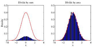
For a probability density function, the integral over the entire space is 1. The previous accepted answer will not give you the correct density. To get the right density, you must divide by the area. To illustrate my point, try the following example.


[f,x]=hist(randn(10000,1),50);%# create histogram from a normal distribution.
g=1/sqrt(2*pi)*exp(-0.5*x.^2);%# pdf of the normal distribution

%#METHOD 1: DIVIDE BY SUM
figure(1)
bar(x,f/sum(f));hold on
plot(x,g,'r');hold off

%#METHOD 2: DIVIDE BY AREA
figure(2)
bar(x,f/trapz(x,f));hold on
plot(x,g,'r');hold off

You can see for yourself which method agrees with the correct answer (red curve).


However, for some distributions (like Cauchy) I have found that trapz will overestimate the area, and so the pdf will change depending on the number of bins you select. In this case it is useful to do:
[N,h]=hist(q_f./theta,30000);
% there Is a large range but most of the bins will be empty
plot(h,N/(sum(N)*mean(diff(h))),'+r')

Appendix: Trapezoid integration

Trapezoidal numerical integration in MATLAB is done by the function called trapz.

Syntax

Z = trapz(Y) computes an approximation of the integral of Y via the trapezoidal method (with unit spacing). To compute the integral for spacing other than one, multiply Z by the spacing increment. Input Y can be complex. If Y is a vector, trapz(Y) is the integral of Y. If Y is a matrix, trapz(Y) is a row vector with the integral over each column.

Z = trapz(X,Y) computes the integral of Y with respect to X using trapezoidal integration. Inputs X and Y can be complex.


Example of trapz application

Let's compute the 0πsin(x)dx. The exact value of this integral is 2.

To approximate this numerically on a uniformly spaced grid, use

X = 0:pi/100:pi;

Y = sin(X);

Then use the trapz function:

Z = trapz(X,Y)

that produces:

Z = 1.9998

The result is not as accurate as the uniformly spaced grid [3].


Monday, August 6, 2012

NP Hard problem - explanation from Stephen Boyd

Students used to ask me about this - what is NP-hard problem and why is it important? The exact answer can easily be a topic of a monograph, but I have been looking for a simple yet accurate answer.


Well, NP stands for Non-deterministic Polynomial time. Simply speaking, an NP-complete problem cannot be solved in polynomial time in any known way. NP-Hard/NP-Complete is a way of showing that certain classes of problems are not solvable in realistic time.


Basically, a solution has to be testable in polynomial time. If that's the case, and a known NP problem can be solved using the given problem with modified input (an NP problem can be reduced to the given problem) then the problem is NP complete. NP-complete means the problem is at least as hard as any problem in NP.


On the other hand, there are polynomial-time problems. The class P consists of those problems that are solvable in polynomial time. For example, they could be solved in O(n^k) for some constant k, where n is the size of the input. Simply put, you can write a program that will run in reasonable time.

A decision problem is in P if there is a known polynomial-time algorithm to get that answer. A decision problem is in NP if there is a known polynomial-time algorithm for a non-deterministic machine to get the answer.

There is a good lecture notes about the NP-hard problems [PDF].

A simple and understandable explanation of the NP-hard problem that I like is given by Stephen Boyd:


This explanation is a bit watery, but basically boils down to the following. People identified a bunch of (computationally) very hard problems, to which nobody figured out a polynomial-time algorithm.

When the problem comes in, you measure the size of the data required to describe the problem. Then you look on the number of operations you have to do, and if you can bound that number of computations by polynomial, that's the polynomial-type problem.

There is a catalog of problems that are considered as computationally hard. You can call the problem as NP-hard if it is as hard as any of the problems from that catalog (e.g., travelling salesman).
Related Posts Plugin for WordPress, Blogger...