Normalised histogram calculations
The usual approximation for the probability density function is a histogram. The probability density function is non-negative everywhere, and its integral over the entire space is equal to one [1]. Formally, a random variable X has density f, where f is a non-negative Lebesgue-integrable function, if:
\operatornameP[a ≤ X ≤ b]=∫abf(x)\,\mathrm{d}x.
There are many ways to normalise the histogram, and some of those methods have limitations. Consider all of them.
Normalisation by sum
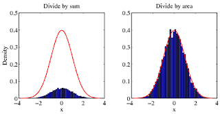
This solution answers the question How to have the sum of all bins equal to 1. The example of code is here:
[f,x]=hist(randn(10000,1),50);%# create histogram from a normal distribution.
g=1/sqrt(2*pi)*exp(-0.5*x.^2);%# pdf of the normal distribution

%#METHOD 1: DIVIDE BY SUM
figure(1)
bar(x,f/sum(f));hold on
plot(x,g,'r');hold off
This approximation is valid only if your bin size is small relative to the variance of your data [2]. The sum used here correspond to a simple quadrature formula, more complex ones can be used like trapz.
Normalisation by area
For a probability density function, the integral over the entire space is 1. The previous accepted answer will not give you the correct density. To get the right density, you must divide by the area. To illustrate my point, try the following example.
[f,x]=hist(randn(10000,1),50);%# create histogram from a normal distribution.
g=1/sqrt(2*pi)*exp(-0.5*x.^2);%# pdf of the normal distribution

%#METHOD 1: DIVIDE BY SUM
figure(1)
bar(x,f/sum(f));hold on
plot(x,g,'r');hold off

%#METHOD 2: DIVIDE BY AREA
figure(2)
bar(x,f/trapz(x,f));hold on
plot(x,g,'r');hold off
You can see for yourself which method agrees with the correct answer (red curve).

However, for some distributions (like Cauchy) I have found that
trapz will overestimate the area, and so the pdf will change depending on the number of bins you select. In this case it is useful to do:[N,h]=hist(q_f./theta,30000);
% there Is a large range but most of the bins will be empty
plot(h,N/(sum(N)*mean(diff(h))),'+r')
Appendix: Trapezoid integration
Trapezoidal numerical integration in MATLAB is done by the function called trapz.
Syntax
Z = trapz(Y) computes an approximation of the integral of Y via the trapezoidal method (with unit spacing). To compute the integral for spacing other than one, multiply Z by the spacing increment. Input Y can be complex. If Y is a vector, trapz(Y) is the integral of Y. If Y is a matrix, trapz(Y) is a row vector with the integral over each column.
Z = trapz(X,Y) computes the integral of Y with respect to X using trapezoidal integration. Inputs X and Y can be complex.
Example of trapz application
Let's compute the ∫0πsin(x)dx. The exact value of this integral is 2.
To approximate this numerically on a uniformly spaced grid, use
X = 0:pi/100:pi;
Y = sin(X);
Then use the trapz function:
Z = trapz(X,Y)
that produces:
Z = 1.9998
The result is not as accurate as the uniformly spaced grid [3].